2020-2021 Regular Season Retrospective

July 20, 2021, Micah Blake McCurdy, @IneffectiveMath

Some exposition here is copied from my 2018-2019 Retrospective

Various people have made models to try to predict the outcomes of hockey games, including me. I think the problem is intrinsically interesting, and I find it helpful as a point around which to organize much of my work in hockey. A good model has many aspects, chiefly:

• Sensible methods which give insight into the processes being modelled;
• Interpretability of inputs and outputs; and
• Suitably accurate and precise results.

This article is about the last item.

The models under consideration here are:

• My model, Magnus, published on this site,
• Peter Tanner's model, published at Moneypuck.com,
• Dominik Luszcyzszyn's model, published on his twitter account @domluszczyszyn, (and at The Athletic)
• Matt Chernos's model, published on his twitter account @mchernos,
• The model published on the account of twitter user @hockeystatisti1,

For models that output probabilities, there is no sensible way to say that a model is "right" or "wrong", such binary judgments apply to binary choices which these models do not make. Instead, I use using "logarithmic loss", that is, assigning a score of -ln p to an event which occurs and which was predicted to occur with probability p. This loss function is called "logarithmic" because it is defined with the natural logarithm function (ln) and is is commonly abbreviate to "log-loss". I like log-loss best because it is the only scoring rule which, if the people estimating the probabilities know that it will used ahead of time to judge them, incentivizes them to quote probabilities which exactly match their certainty of the events in question occurring.

The obvious benchmark for a model of probability is to simply say that the home team has a 50% chance of winning every game, this gives a log-loss of -ln 0.5 ≈ 0.693. A supremely confident prediction that a team will win with a chance of 99% gives a log-loss, if correct, of -ln 0.99 ≈ 0.01, and if incorrect, of -ln 0.01 ≈ 4.605. Scores close to 0 are "not at all wrong", and high scores are "very wrong". However, the benchmark value of 0.693 is not one that sticks in the mind and the lower scores being better is confusing. In an effort to make log-losses more understandable, I apply a linear scaling to map 0.693 to 50 and 0 to 100. This makes log-loss behave like a test score - fifty is the passing grade, and a hundred is a perfect score. However, unlike test scores, models with extremely bad predictions can score below zero (and one or two games from one or two models this year did score below zero). I call this "log-loss-as-test-score", for lack of a better name; and every prediction is its own little test, graded by the outcome of the game.

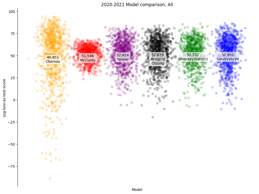
Each point displayed is an individual game of the 2020-2021 season, with its log-loss-as-test-score for each model. Most obviously, most models are slightly better than the guessing benchmark of 50 points, and the differences between models in overall performance are quite small. More interestingly, despite the overall similarities in results, each model has a considerable spread in results. Some models, like mine especially, are by nature conservative, assigning probabilities close to 50%. Others, like Dominik Luszczyszyn's, are more extravagant, assigning probabilities far from 50% more often.

For a more difficult task than simply out-peforming a person guessing, I've also included probabilities corresponding to (approximately de-vigorished) Pinnacle closing lines, helpfully supplied for almost all games by Matt Chernos.

Calibration

In addition to game-by-game accuracy, we would like our predictive models to be well-calibrated; that is, for any sufficiently-large set of games we would like the predicted percentage of winners to closely match the observed percentage of winners. I have two methods of forming such sets today: binning the games by home-team win probability and binning them by time.

Deciles of Risk

One common calibration measure is to form so-called "deciles of risk", that is, sorting all of the winning team probabilities (not the home team probabilities) for each model from lowest to highest, binning them into ten bins, and comparing the predicted probabilities for each bin to the proportion of home team wins in each bin.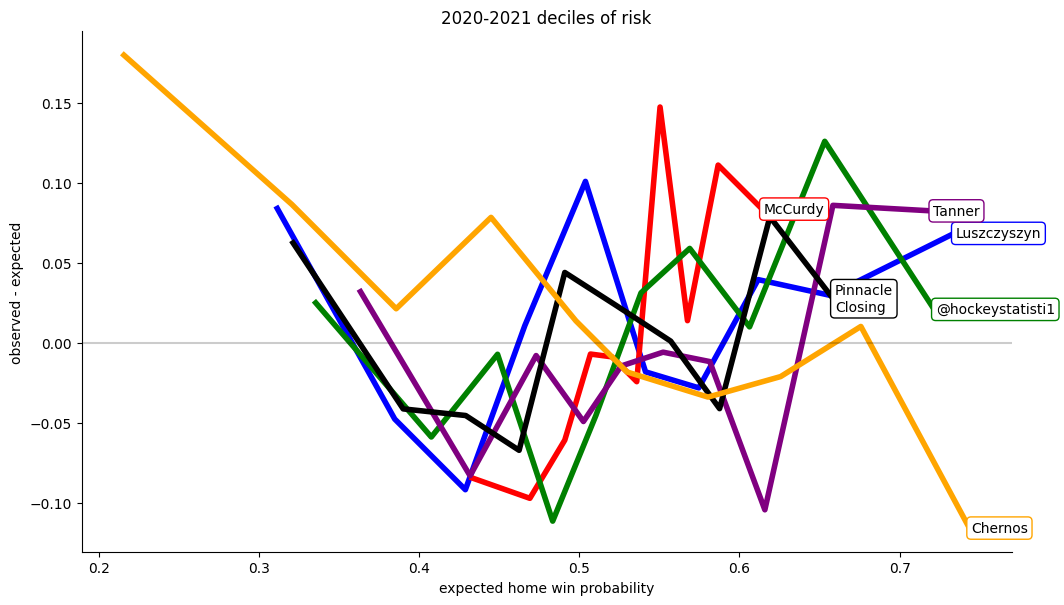
For models without structural defects, these differences should be randomly distributed around zero, as several of the models considered here are. However, it is impossible to miss that my model specifically (the red line) is calibrated poorly; It's not sure enough when backing winners and not sure enough when fading losers.

Time Calibration

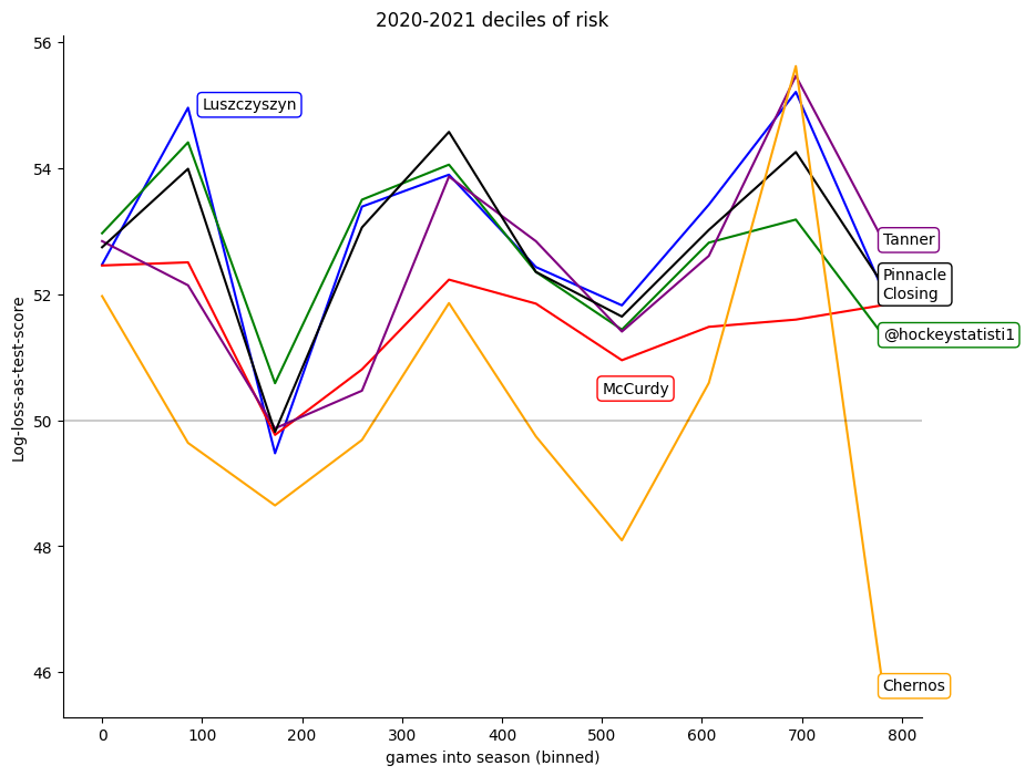
Alternatively, we can sort the games by their playing date, and then compare the calibration of the models over time. Here the striking feature is how similar to one another many of the models are. Here again my model is the one that stands out for being unusual; dipping where all the others rise near the end of the season.

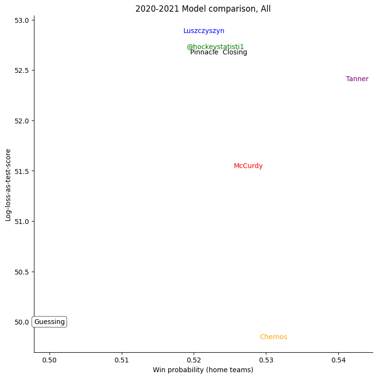
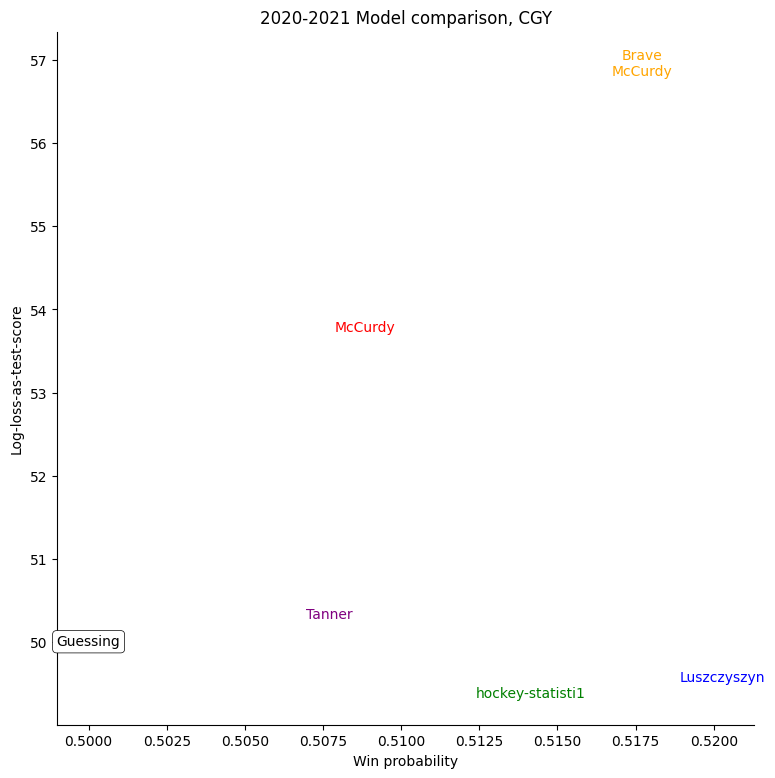
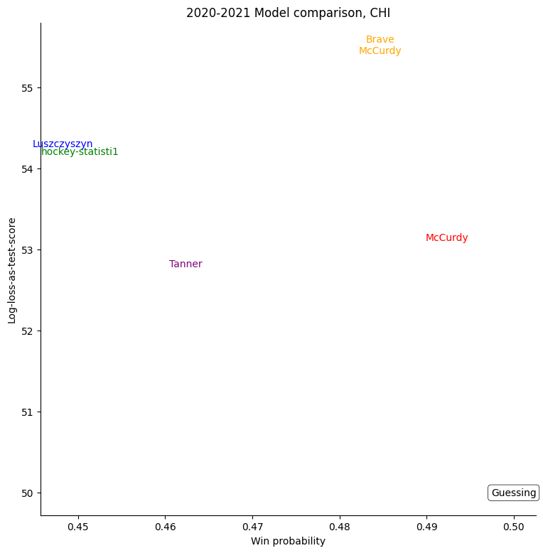
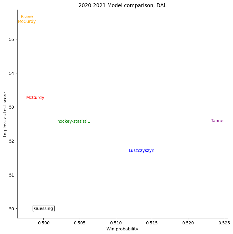
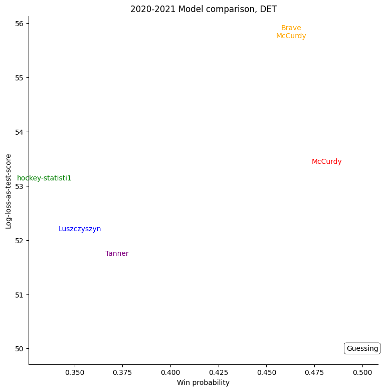
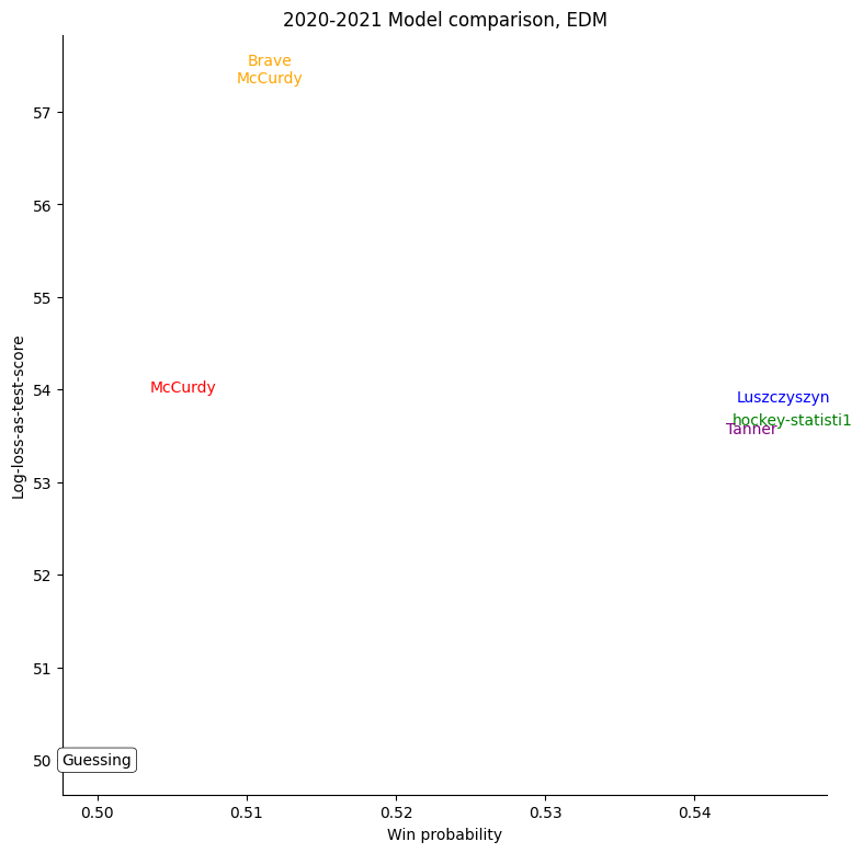
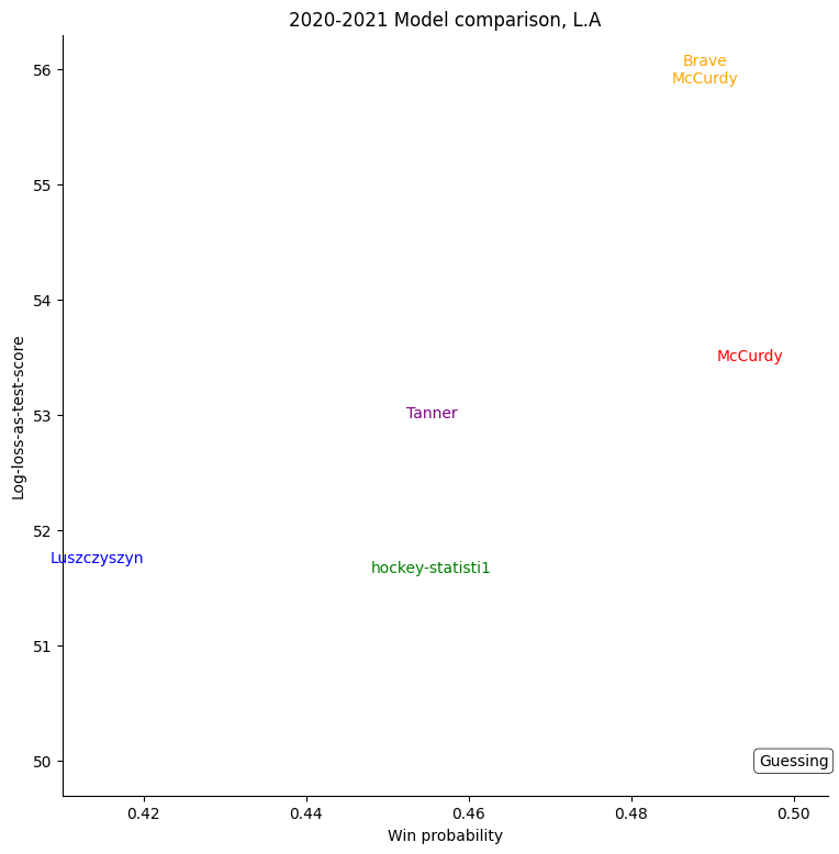
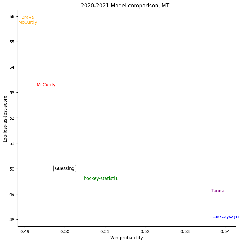
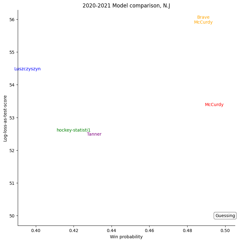
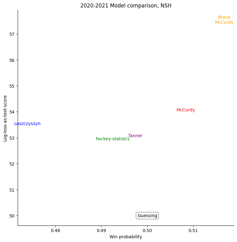
Probability vs Log-loss

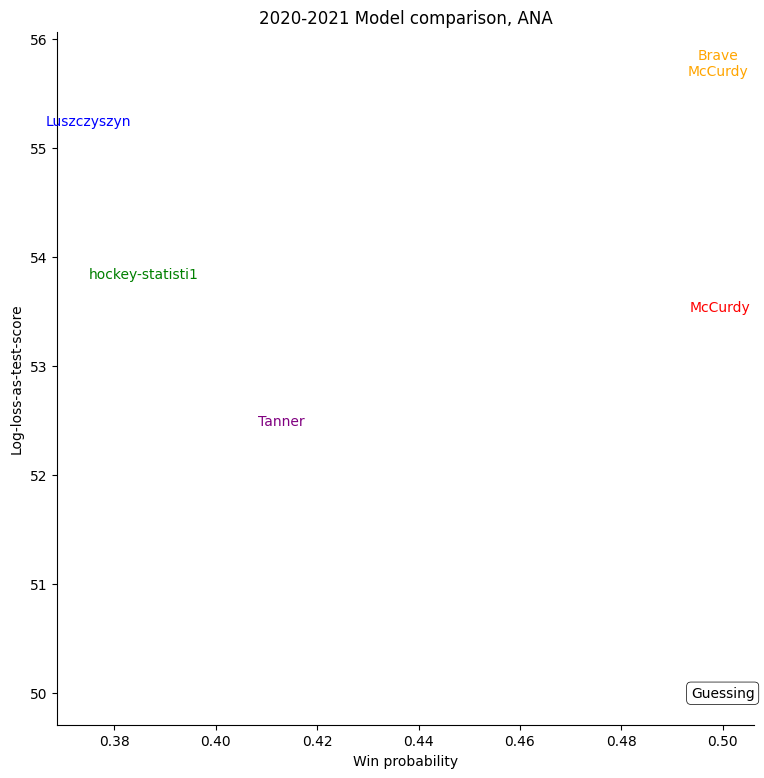
To see just where individual models went wrong, it's helpful to consider a set of teams and compare the probabilities given to the log-losses for those teams. First of all, we can consider all home-teams:

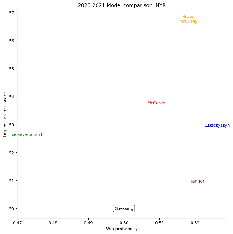
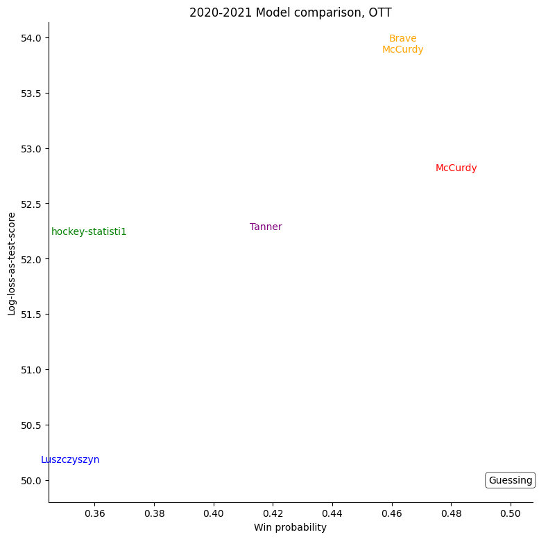
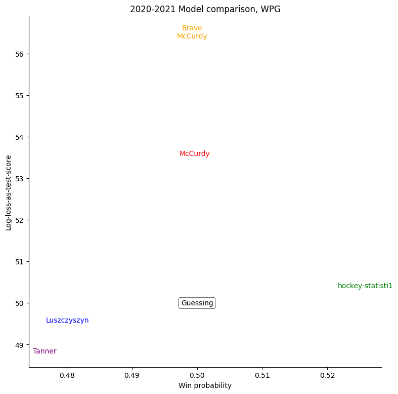
Team-by-team Results

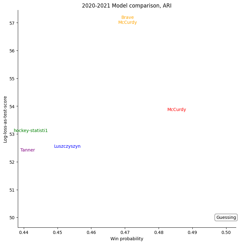
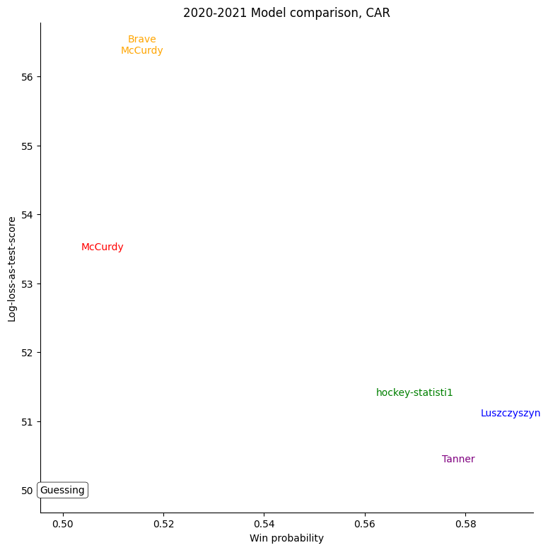
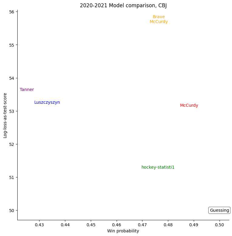
The same exercise can be repeated for each individual team, shown in the table below.

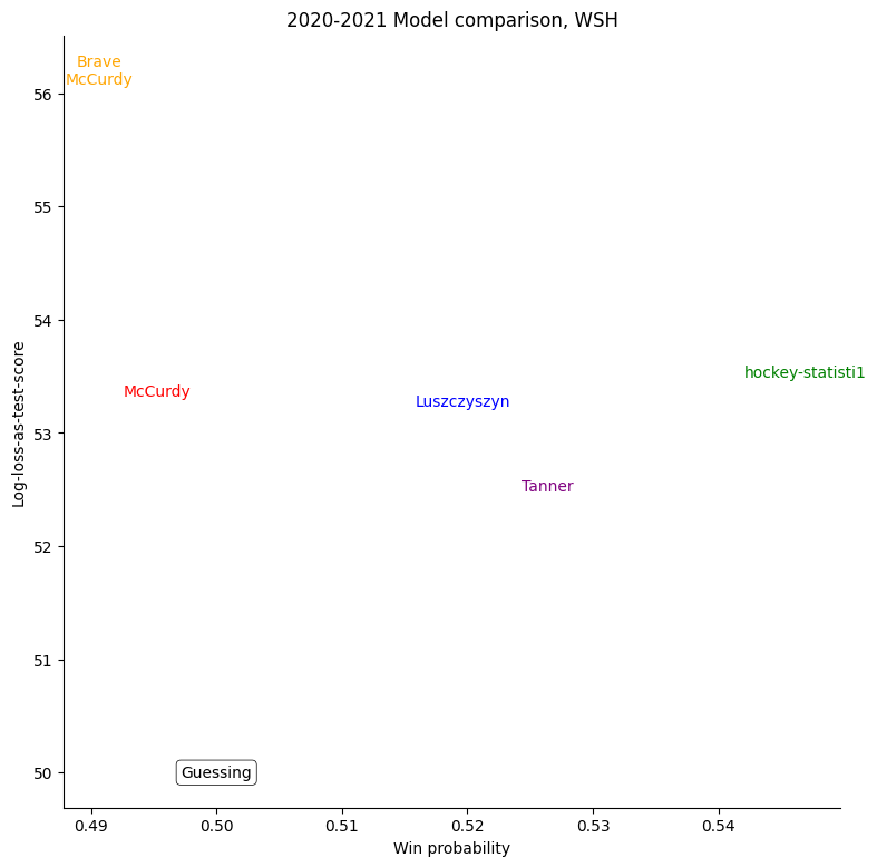
For some very successful teams, like Colorado, Vegas, or Tampa, an easy way to score highly was to back them very strongly. For other, very unsuccessful teams, like Buffalo, the easy way to score highly was to strongly back their opponents. Most other teams don't show a clear "underrate"/"overrate" pattern.

---