Estimating Individual Impact on NHL 5v5 Shot Rates
(I discussed a closely related precursor to this portion of Magnus at the 2018 Ottawa Hockey Analytics Conference, of which you can read the slides.)
I would like to be able to isolate the individual impact of a given skater on shot rates from the impact of their teammates, their opponents, the scores at which they play, the zones in which they begin their shifts, and home-ice advantage. I have fit a regression model which provides such estimates. The most important feature of this model is that I use shot rate maps as the units of observation and thus also for the estimates themselves, permitting me to see not only what portion of a team's performance can be attributed to individual players but also detect patterns of ice usage.
Here, as throughout this article, "shot" means "unblocked shot", that is, a shot that is recorded by the NHL as either a goal, a save, or a miss (this latter category includes shots that hit the post or crossbar). I would prefer to include blocked shots also but cannot since the NHL does not record shot locations for blocked shots.
The most sophisticated element of Magnus is the method for estimating the marginal effect of a given player on shot rates; that is, that portion of what happens when they are on the ice that can be attributed to their individual play and not the context in which they are placed. We know that players are affected by their teammates, by their opponents, by the zones their coaches deploy them in, and by the prevailing score while they play. Thus, I try to isolate the impact of a given player on the shots which are taken and where they are taken from.
Although regression is mathematically more sophisticated than some other measures, it is in no way a "black box". As we shall see, every measurement can be broken down into its constituent pieces and scrutinized. If you are uneasy with the mathematical details but interested in the results, you should skip the "Method" section and just think of the method as like a souped-up "relative to team/teammate statistics", done properly.
Method
I use a simple linear model of the form \( Y = WX\beta \) where \(X\) is the design matrix, \(Y\) is a vector of observations, \(W\) is a weighting matrix, and \(\beta\) is a vector of marginals, that is, the impacts associated to each thing independent of each other thing.
The columns of \(X\) correspond to all of the different features that I include in the model. There are five different types of columns:
- Player performance estimates, two columns for each skater: one for their offensive impact (that is, on their own team's shot rates), and one for their defensive impact (that is, on their opponent's shot rates);
- Score impacts: six columns for various different scores: trailing by three or more, trailing by two, trailing by one, leading by one, leading by two, and leading by three or more. There is no column for tied, which is taken as the reference state;
- Zone impacts: eight columns for the zones in which players start their shifts. The
four "shift start types" that I use are:
- Offensive Zone,
- Neutral Zone,
- Defensive Zone, and
- On-the-fly Starts.
- Intercept: one column to indicate home-ice advantage.
The entries in \(Y\) are functions which encode the rate at which unblocked shots are generated from various parts of the ice. An unblocked shots with NHL-recorded location of \((x,y)\) is encoded as a two-dimensional gaussian centred at that point with width of ten feet; this arbitrary figure is chosen because it is large enough to dominate the measurement error typically observed by comparing video observations with NHL-recorded locations and also produces suitable smooth estimates.
One detailed example should make the structure of the model clear:
Suppose that the Senators are the home team and the Jets are the away team, and at a given moment of open play two Senators players (say, Karlsson and Phaneuf) jump on the ice, replacing two other Senators. The score is 2-1 for Ottawa, and the other players (say, Pageau, Hoffman, and Stone for Ottawa, against Laine, Ehlers, Wheeler, Byfuglien, and Enstrom) began their shift some time previously on a faceoff in Ottawa's zone. Play continues for 50 seconds, during which time Ottawa takes two unblocked shots from locations (0,80) and (-10,50) and Winnipeg takes no shots. This shift ends with the period and the players leave the ice.
These fifty seconds are turned into two rows of \(X\) and two entries in \(Y\). First, the Ottawa players are considered the attackers, and the attacking columns for Pageau, Hoffman, Stone, Karlsson, and Phaneuf are all marked as "1". The Jets are considered the defenders and the defending columns for Laine, Ehlers, Wheeler, Byfuglien, and Phaneuf are marked as "1". All of the other player columns, attacking or defending, are marked as "0". Because the Senators are winning 2-1, the score column for "leading by one" is marked with a "1" and the other score columns are marked as "0". Because three of the Senators players are playing on-the-fly shifts, and the Senators are the home team, the "home on-the-fly attacking" zone column is marked with "0.6", because sixty percent of the five players are playing such shifts. The other two Senators players are still playing the shift they began in their own zone, so the "home defensive-zone attacking" zone column is marked with "0.4". All of the jets skaters began their shift in the Ottawa zone, so the "away offensive-zone defending" zone column is marked with a "1.0", and all the other zone columns are marked as "0". The Senators are the home team, so the "home intercept" column is marked with a 1. Corresponding to this row of \(X\), an entry of \(Y\) is constructed as follows: Two gaussians of ten-foot width and unit volume are placed at (0,80) and (-10,50) and the two gaussians are added to one another. This function is divided by fifty; resulting in a continuous function that approximates the observed shot rates in the shift. Finally, I subtract the league average shot rate from this. This function, which associates to every point in the offensive half-rink a rate of shots produced in excess of league average from that location, is the "observation" I use in my model.Second, the same fifty seconds are made into another observation where the Jets players are considered the attackers, and the Senators are the defenders. The attacking player columns for the Jets are set to 1, the defending columns for the Senators players are set to 1. Since the Jets are losing, the score column of "trailing by one" is set to 1, and the non-zero zone columns are:
The two rows have no non-zero columns in common. Since the Jets didn't generate any shots, the associated function is the zero function; I subtract league average shot rate from this and the result is placed in the observation vector \(Y\).
- "away offensive zone attacking": 1.0
- "home on-the-fly defending": 0.4
- "home defensive zone defending": 0.6
The weighting matrix \(W\), which is diagonal, is filled with the length of the shift in question. Thus, the above two rows will each have a weight of fifty.
By controlling for score, zone, teammates, and opponents in this way, I obtain estimates of each players individual isolated impact on shot generation and shot suppression.
To fit a simple model such as \(Y = WX\beta \) using ordinary least squares fitting is to find the \(\beta\) which minimizes the total error $$ (Y - X\beta)^TW(Y - X\beta) $$ When the entries of \(Y\) are numbers, this expression is a one-by-one matrix which I naturally identify with the single number it contains, and I can find the \(\beta\) which minimizes it by the usual methods of matrix differentiation. To extend this framework to our situation, where the elements of \(Y\) are functions from the half-rink to the reals, I must define an inner product on this function space, which I do by setting \( \left< f,g \right> = \int f(x,y) g(x,y) dA \) where the integral is taken over all coordinates \((x,y)\) in the half rink. Since I only use functions which are finite sums of gaussians, this integral always exists and is easily checked to define an inner product. Hence, I can use the well-known formula for the \(\beta\) which minimizes this error, namely $$ \beta = (X^TX)^{-1}X^TWY $$ which makes it clear that the units of \(\beta\) are the same as those of \(Y\); that is, if I put shot rate maps in, I will get shot rate maps out.
However, I choose not to fit this model with ordinary least-squares, preferring instead to use generalized ridge regression; that is, I choose to minimize $$ (Y - X\beta)^TW(Y - X\beta) + \beta^T \Lambda \beta $$ where \(\Lambda\) is a positive definite matrix which encodes our prior knowledge about the players. This is a kind of zero-biased regression---the first error term is as before, but the second term, weighted by \(\Lambda\), interprets deviation from zero (that is, league average) as intrinsically mistaken. The \(\beta\) which minimizes this combined expression is the one which simultaneously agrees with the observations while doing as little violence as possible to the idea that the players in question are all, broadly, of NHL quality.
The usual methods (that is, differentiating with respect to \(\beta\) to find the unique minimum of the error expression) gives a closed form for \(\beta\) as: $$ \beta = (X^TWX + \Lambda)^{-1}X^TWY $$ Any positive definite \(\Lambda\) will suffice but I choose to use a simple diagonal one, with entries \(\Lambda_{ii} = \lambda_i\) depending on the column \(i\) as follows:
- For the score columns and the home-ice intercept, I choose \(\lambda = 0\). These terms are not theoretically constrained.
- For the zone columns, I choose \(\lambda = 0.001\), that is, as close to zero as possible without causing grief to my smoothing algorithm.
- For all other terms (for players, zones, and scores) I use \(\lambda = 10,000\). This value is obtained by examining the estimates for various \(\lambda\) and choosing a sufficiently high value for stable, slowly varying estimates. More involved theoretical estimates of which \(\lambda\) ought to be best (such as computing the generalized cross-validation error, following Brian MacDonald (Section 5.3)) suggest must smaller \(\lambda\) values which give wildly varying year-to-year estimates of player ability.
- For players with fewer than a thousand minutes of 5v5 icetime in a given season, I linearly scale the associated \(\lambda\) by the fraction of a thousand minutes the player has played, down to a minimum of 2,000. Theoretically, I justify the choice of ridge regression by appealing (faintly) to the gate-keeping ability of coaches and managers who determine icetime. However, players with few minutes do not come with such strong guarantees of NHL-average ability as those with many minutes whose coaches are presumably sure of them. In every case the introduced bias is towards zero (that is, league average) but players with little icetime are more loosely bound to this initial estimate. This permits the large multiplicity of largely below-average players who move up and down through the league to be given the weak estimates they deserve and also permits very young players who are nevertheless unusually good (as several are each season) to be recorded as such despite not having the age required to be known-as-good to their coaches.
One tantalising possibility for the future is that expected chemistry effects might be encoded in more subtle choices of \(\Lambda\) - for instance, if one expected ahead of time that player i and player j were going to produce similar results, one could set \(\Lambda_{ij}\) to be negative (instead of zero as above), effectively penalizing any differences between them. This is only the germ of a tiny idea but the Sedins come immediately to mind.
Results
For the purposes of examining the distribution of estimates, I use a simple "expected goals" style weighting which I call threat. That is, for a given location, I can calculate the historical chance of a shot (known to be unblocked, as assumed throughout this article) of becoming a goal, without paying attention to any other features of the shot.

The model can be fit to any length of time; in this article I'll be describing the results from fitting the 2016-2017 and 2017-2018 regular seasons together, since these results are the ones which I used for my 2018-2019 season preview. Eventually, single-season results will be posted in relevant spots throughout the site.
Raw on-ice results
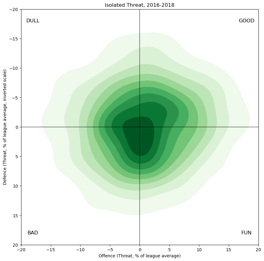
Before I describe the model outputs, I turn first to the raw observed results from the combined 2016-2018 regular seasons.

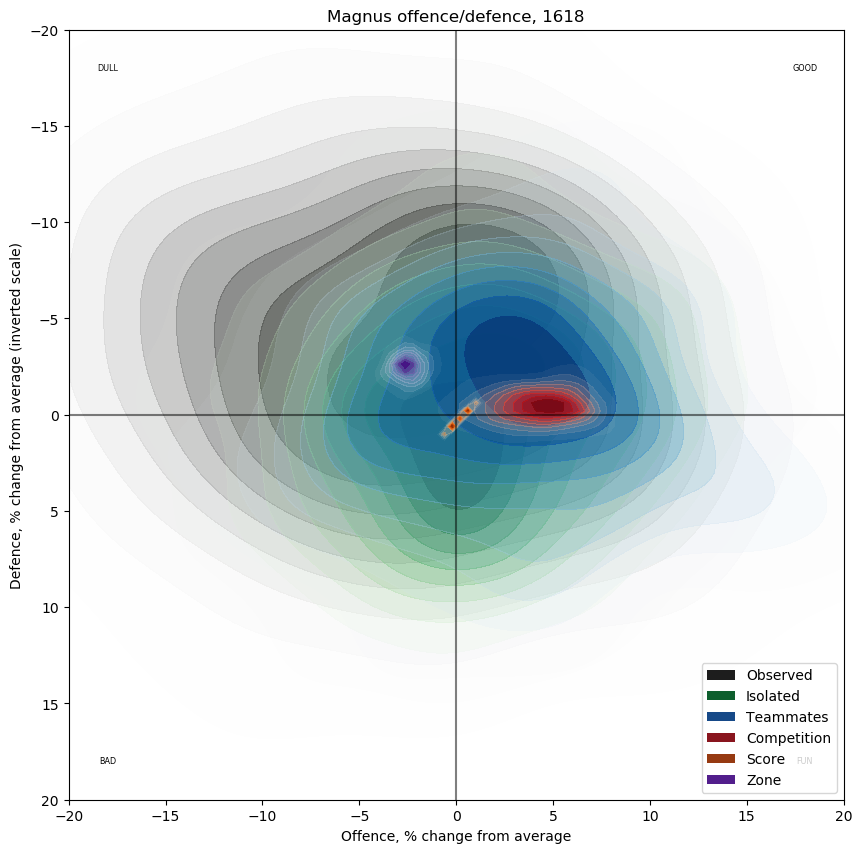
This graph is constructed as follows: for every skater who played any 5v5 minutes in these two seasons, compute the offensive and defensive threat observed while they were on the ice; this produces a point \(x,y\). Then, form the density map of all such points, where each point is weighted by the corresponding number of minutes played by the player in question. For ease of interpretation, I've scaled the threat values by league average threat, so that a value of \(5,5\) on the graph means "threating to score 5% more than league average, and also threatening to be scored on 5% more than league average". As is my entrenched habit, the defensive axis is inverted, so results that are favourable to the skater in question appear in the top right. The contours are chosen so that ten percent of the point mass is in the darkest region, another ten percent in the next region, and so on. The final twenty percent of the point mass is in the white region surrounding the shaded part of the graph.
Player Marginals
Repeating the above process with the individual player marginal estimates gives the following graph in green. Unsurprisingly, since I used a model with an explicit zero-bias, the overall distribution is roughly normal around zero. Intuitively, we expect this means that weak players will be slightly over-estimated and that strong players will be under-estimated; I hope in this way to obtain the clearest possible view of players whose true ability is close to league average---these players interest me a great deal more than the other players. The choice of zero-point for the regression is mathematically arbitrary, so its choice is determined by ease of interpretability and by which sorts of players are of interest---akin to moving a magnifying glass over a large map, knowing that the fine details in the centre will be easier to see but the areas under the edges of the glass distorted.
Notice also that there is no correlation between offensive ability and defensive ability, which confirms previous work by me. There are certainly many players who are offensively strong and defensively weak, but it does not appear to govern play like the tired cliche suggests.
Teammate Impact
Once I have individual estimates for players in hand, I can make many interesting secondary computations to show the distribution of various effects. Most obviously, for a given player, I can form the sum of the player estimates of all the given player's teammates, weighted by their shared icetime, and then multiply it by four (since every player has four teammates at 5v5). These estimates of teammate quality can then be graphed as above:

Here we see a definite skew towards good players; that is, most players are playing with better than average players. This fits our intuition, since better players play mostly with one another and also play considerably more minutes than weaker players when coaches are making rational decisions, which is most of the time.
Opponent Impact
The same computation can be done for any given players 5v5 opponents: form the sum of all of their isolates, weighted by head-to-head icetime, and then multiply by five, since every player has five opponents at 5v5. This is graphed below in red:

First, notice that the scale on the axes is smaller than for teammates; more discussion of that will follow later. More interestingly, this distribution is both sharply skewed and non-symmetrical. Opponent distributions are skewed broadly towards good players (as for teammates, for similar reasons) but the skew is much more pronounced in the offensive direction; that is, matchups against good offensive players are more common. Furthermore, the variation in competition quality is much more pronounced offensively, with some players playing against skaters of near-average offensive ability but others playing against very strong offensive players. By contrast, the range of defensive ability faced by players is much smaller.
Score and Zone Impact
There is one minor but slightly unusual bit of technical sleight-of-hand which I must explain here. One of the model columns is a home-ice advantage term, which does several things simultaneously---it plays a role analogous to the "tied" score state, which does not have a column to itself, it obviously measures in some very imprecise way some of the effect of home-ice advantage (I hope presumptively that modelling teammates and competition explicitly also captures some), and it serves as a reservoir into which any unmodelled effects can partially fall. Since it must do so many things, I have decided to include it partially in the score impacts and partially in the zone impacts, in a slightly ad-hoc way, as we shall see. For reference, the home-ice term is the following:

Score
The score terms for 2016-2018 are as follows:

As is by now familiar, teams which are losing dominate games in shots and goals, although they still usually lose. Curiously for 2016-2018, all of the "losing" states are broadly similar, with very little difference in the offence generated by teams that are losing slightly versus ones that are trailing by a large margin. On the other hand, leading teams show a more modest (negative) effect on their shot rates, with a slight bump in shots from the middle of the ice at the expense of shots from the points and perimeter.
To examine how the score affects player results, I form weighted sums of each of these maps, weighted by the fraction of their total icetime (including tied scores, for which there is no covariate). Furthermore, I compute each player's individual home-ice advantage, that is, I multiply the above home-ice covariate by the fraction of their individual ice-time which was spent on home ice. I then add -0.25(this will be explained below) times this amount to the score computation, to obtain their net score impact, which is shown below in orange:

Note that the distribution is quite linear---coaches have very little leeway in score deployment, since given score states tend to prevail for a long time compared to how long it takes players to rest.
Zone
Each player has their own zone start, so the net effect of zone starts for a given shift is computed by adding all of the various individual impacts together. The zone columns themselves are:
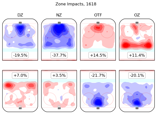
These are scaled for display so that, for instance, if all five skaters on one team were starting their shifts in the defensive zone, the impact on shot rates for that team would be as shown in the "defensive zone" column. The full impact of zone starts on the play can be found by adding the effect for one team to the effect for the other team; this requires some care and attention since defensive zone starts for one team need not correspond with offensive zone starts for the other team. In general, the zone starts for one team are not theoretically required to have anything to do with those of the other team, since each team's players change entirely when their coach desires them to change; however, certain patterns (offensive vs defensive, neutral vs neutral, on-the-fly vs on-the-fly) are more common.
To obtain the distribution of zone impacts on skaters in 2016-2018, I compute the sum of the associated zone impacts of the ten zone starts for the skaters on the ice using the above set of eight estimates, and then add 1.25 times the home-ice advantage of each player to obtain the net zone impact, below in purple:
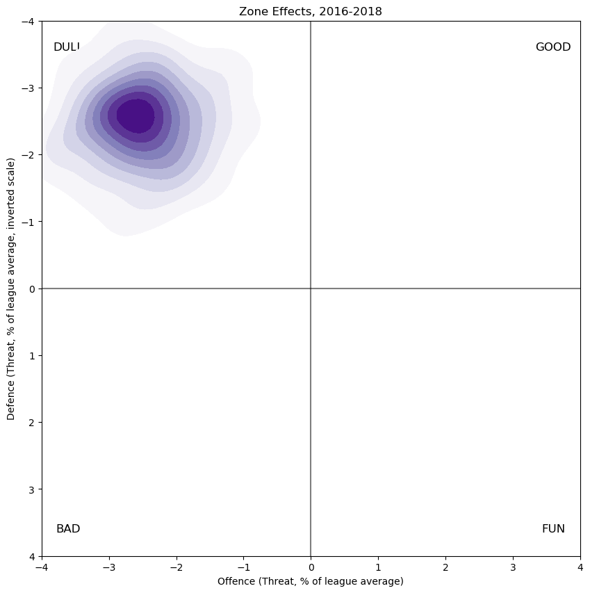
The most obvious thing here is not the clear gaussian shape but the heavy skew towards fewer shots---fewer for both teams. First of all, I must explain the mysterious magic numbers -0.25 and 1.25 which appear in the two preceding paragraphs, which requires a small technical digression. Had I included an overall intercept column alongside the ones I did use, then the columns of the design matrix would have been linearly dependent; specifically, the "down 1", "up 1", "home ice", and "overall intercept" columns would have been linearly dependent, which means that they would have been redundant. Had we been doing ordinary least squares regression, this would have caused our problem to be ill-conditioned and therefore unsolvable. Ridge regression provides a way out of this technically, but it offends my sense of judgment to use non-zero ridge parameters for these columns since there is no theoretical (that is, hockey) reason for these terms to be close to zero. The effect of having a subset of linearly dependent columns in a regression is analogous to trusting a drop of water on a wide, hot flat saucepan to find the lowest point simply by gravity---since the pan is almost totally flat, the water will skitter about and never settle down. (In fact, the origin of the word "ridge" in the sense of ridge regression comes from a similar metaphor, where a "mountain ridge" is added to a "flat" section of configuration space).
Thus, with no clear indication of how to divide the observed home-ice advantage into its manifesting parts, I choose to artificially divide it as I have done (-0.25 to score, 1.25 to zone) purely to (roughly) align the score distribution with the origin, which seems plausible to me. Of course the two coefficients must add to one, the net effect of which moves the zone impact distribution closer to the origin than it was before any home-ice impact is considered.
The most obvious interpretation of this skew towards "DULL" is that changes of player personnel are, in general, associated with decreases of shot rates, which is broadly what we know intuitively happens, especially for faceoff starts, where all ten skaters are usually stationary. Moreover, we know quantitatively that shift starts, including on-the-fly shifts but especially faceoff shifts, begin with depressed shot rates.
"Residuals"
Strictly speaking, residuals for a regression refer to the differences between the individual observations (that is, each microshift, for 2016-2018 about a million or so) and the predicted shot rates for each microshift. I find it prohibitive to compute such residuals, so instead I settle for a suitable aggregate: for each player, I can compute the difference between their raw observed 5v5 on-ice results and what I would expect from computing the model outputs associated with the observed players and the zones and scores and home-ice advantage they player under. This is shown below:
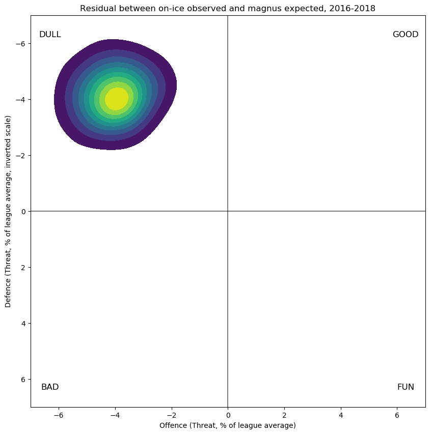
Here again the skew towards "DULL" is the obvious, salient feature---that is, the model predicts more shots than in fact occur, for both teams. I think, but am not certain, that this is because the offensively strong players are so offensively strong that when they play both with and against one another, as the above exposition shows that they disproportionately do, there simply isn't enough time in single shifts for both teams to put up the shot totals that their results against weaker opponents suggest they are capable of doing. If this is true, and again I add that I am not certain, it would be the first suggestion that I have seen that offence and defence might not be independent at the team level, at least in certain shifts.
Relative Scale
In the above, I have shown each distribution on its own scale, so that I could discuss the shape of each one in turn. However, to understand their relative importance, they should all be placed on the same scale, which I have done below (except the residuals):
Here there are a great many interesting insights to be had:
- The spread of talent (green) is much smaller than the spread of observed performances (black). This is partly pre-ordained by the regression choice (since I insisted that the player estimates not deviate too much from zero) but also indicative of how sometimes players and circumstances align to produce (relatively) extreme outcomes compared to the abilities of individuals.
- The teammate distribution is much bigger than the competition distribution, in agreement with many previous studies showing that variation in competition (which is only loosely controlled by coaches) is much smaller than the variation in teammates, which coaches control almost completely. However, there are certain players for whom the net impact of competition is much larger than that of teammates, even over the scale of full seasons. In general, a careful analysis should always begin with teammates but also include competition and contextual effects.
- Controlling for teammates, competition, and zone effects, as we do, the aggregate size of score effects is surprisingly small---almost negligible. This contradicts my previous work on this subject. (The link is to slides for a talk I gave some years ago in Washington; in retrospect the work is shoddy and circularly argued. It is perhaps little wonder that I never wrote it up.)
- Zone effects are also surprisingly small; their total extent is perhaps three or four times smaller than competition effects which are themselves about as much smaller than teammate effects. By focussing on only offensive zone faceoffs and defensive zone faceoffs, as some analyses do, differences between contexts which are in fact quite small can appear heavily inflated.
- Abbott, Spencer
- Abdelkader, Justin
- Åberg, Pontus
- Acciari, Noel
- Agostino, Kenny
- Aho, Sebastian
- Aho, Sebastian
- Alt, Mark
- Alzner, Karl
- Amadio, Michael
- Anderson, Josh
- Andersson, Lias
- Andersson, Rasmus
- Andreoff, Andy
- Andrighetto, Sven
- Anisimov, Artem
- Antipin, Viktor
- Archibald, Darren
- Archibald, Josh
- Armia, Joel
- Arvidsson, Viktor
- Aston-Reese, Zachary
- Athanasiou, Andreas
- Atkinson, Cam
- Auger, Justin
- Austin, Brady
- Auvitu, Yohann
- Backes, David
- Backlund, Mikael
- Bäckström, Nicklas
- Baertschi, Sven
- Bailey, Casey
- Bailey, Josh
- Bailey, Justin
- Balisy, Chase
- Baptiste, Nicholas
- Barbashev, Ivan
- Barberio, Mark
- Barber, Riley
- Barkov, Aleksander
- Barrie, Tyson
- Bartkowski, Matt
- Barzal, Mathew
- Bass, Cody
- Beagle, Jay
- Bear, Ethan
- Beauchemin, Francois
- Beaulieu, Nathan
- Beauvillier, Anthony
- Beck, Taylor
- Beleskey, Matt
- Bellemare, Pierre-Édouard
- Belpedio, Louis
- Bennett, Beau
- Bennett, Sam
- Benning, Matthew
- Benn, Jamie
- Benn, Jordie
- Bergeron, Patrice
- Berglund, Patrik
- Bernier, Steve
- Bertschy, Christoph
- Bertuzzi, Tyler
- Bickell, Bryan
- Biega, Alex
- Bieksa, Kevin
- Bigras, Chris
- Bitetto, Anthony
- Björk, Anders
- Bjorkstrand, Oliver
- Bjugstad, Nick
- Blais, Samuel
- Blandisi, Joseph
- Blidh, Anton
- Blunden, Mike
- Bødker, Mikkel
- Boeser, Brock
- Bogosian, Zach
- Boll, Jared
- Bonino, Nick
- Booth, David
- Borgman, Andreas
- Borgström, Henrik
- Borowiecki, Mark
- Bortuzzo, Robert
- Boucher, Reid
- Bouma, Lance
- Bournival, Michael
- Bourque, Gabriel
- Bourque, Rene
- Bouwmeester, Jay
- Bowey, Madison
- Boychuk, Johnny
- Boyd, Travis
- Boyle, Brian
- Bozak, Tyler
- Brassard, Derick
- Bratt, Jesper
- Braun, Justin
- Brickley, Connor
- Brickley, Daniel
- Broadhurst, Alex
- Brodin, Jonas
- Brodie, T.J.
- Brodzinski, Jonny
- Brodziak, Kyle
- Brouwer, Troy
- Brown, Connor
- Brown, Dustin
- Brown, J.T.
- Brown, Logan
- Brown, Patrick
- Buchnevich, Pavel
- Burakovsky, Andre
- Burgdoerfer, Erik
- Burmistrov, Alex
- Burns, Brent
- Burrows, Alex
- Butcher, Will
- Butler, Chris
- Byfuglien, Dustin
- Byron, Paul
- Caggiula, Drake
- Callahan, Mitchell
- Callahan, Ryan
- Calvert, Matthew
- Cammalleri, Mike
- Campbell, Brian
- Cannone, Patrick
- Capobianco, Kyle
- Carey, Paul
- Carle, Matt
- Carlo, Brandon
- Carlsson, Gabriel
- Carlson, John
- Carpenter, Ryan
- Carrier, Alexandre
- Carrick, Connor
- Carrick, Trevor
- Carrier, William
- Carr, Daniel
- Carter, Jeff
- Catenacci, Daniel
- Cave, Colby
- Ceci, Cody
- Cehlarik, Peter
- Chabot, Thomas
- Chaput, Michael
- Chára, Zdeno
- Chiarot, Ben
- Chiasson, Alex
- Chimera, Jason
- Chlapík, Filip
- Chorney, Taylor
- Chychrun, Jakob
- Chytil, Filip
- Cirelli, Anthony
- Cizikas, Casey
- Claesson, Fredrik
- Clendening, Adam
- Clifford, Kyle
- Clutterbuck, Cal
- Coburn, Braydon
- Cogliano, Andrew
- Colborne, Joe
- Coleman, Blake
- Cole, Ian
- Comeau, Blake
- Compher, J.T.
- Conacher, Cory
- Condra, Erik
- Connauton, Kevin
- Connolly, Brett
- Connor, Kyle
- Copp, Andrew
- Corrado, Frank
- Cousins, Nick
- Couture, Logan
- Couturier, Sean
- Coyle, Charlie
- Cracknell, Adam
- Cramarossa, Joseph
- Crescenzi, Andrew
- Criscuolo, Kyle
- Crosby, Sidney
- Crouse, Lawson
- Cullen, Matt
- Czarnik, Austin
- Dadonov, Evgeny
- Dahlbeck, Klas
- Dahlström, Carl
- Dal Colle, Michael
- Daley, Trevor
- Dalpe, Zac
- Danault, Phillip
- Daňo, Marko
- Dauphin, Laurent
- Davidson, Brandon
- DeAngelo, Anthony
- Dea, Jean-Sebastien
- DeBrincat, Alex
- DeBrusk, Jake
- De Haan, Calvin
- DeKeyser, Danny
- De La Rose, Jacob
- Del Zotto, Michael
- DeMelo, Dylan
- Demers, Jason
- Dermott, Travis
- Desharnais, David
- Desjardins, Andrew
- Deslauriers, Nicolas
- Despres, Simon
- Dickinson, Jason
- Didomenico, Christopher
- Di Giuseppe, Phillip
- Dillon, Brenden
- Djoos, Christian
- Doan, Shane
- Domi, Max
- Donato, Ryan
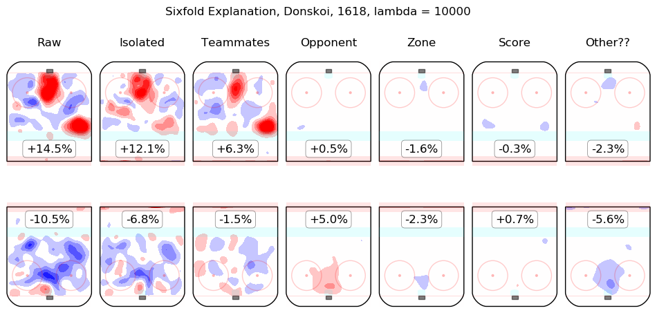
- Donskoi, Joonas
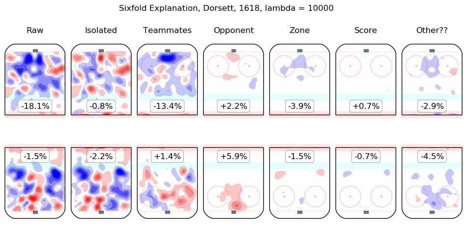
- Dorsett, Derek
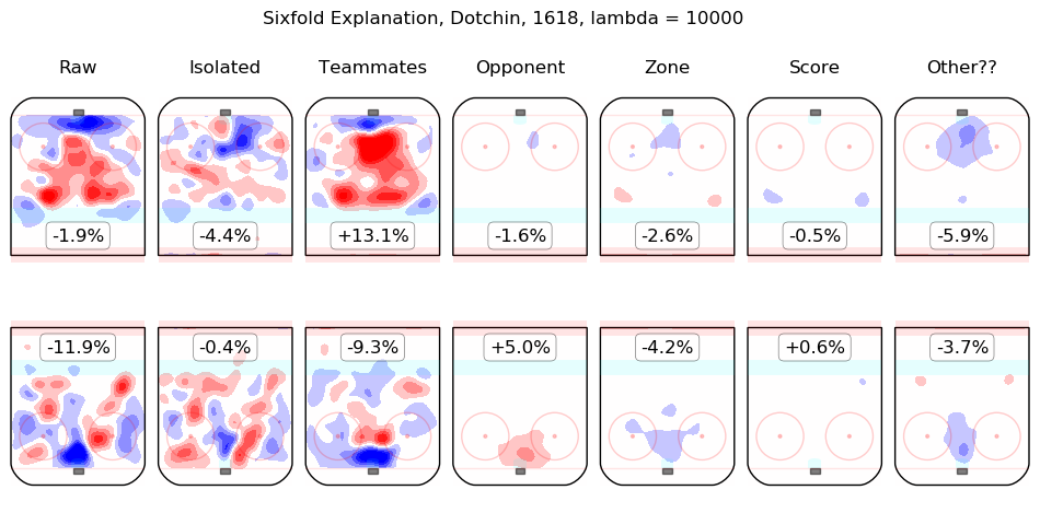
- Dotchin, Jake
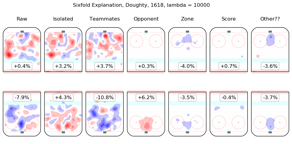
- Doughty, Drew
- Dowd, Nic
- Dowling, Justin
- Draisaitl, Leon
- Drouin, Jonathan
- Dubinsky, Brandon
- Dubois, Pierre-Luc
- Duchene, Matt
- Duclair, Anthony
- Dumba, Matt
- Dumont, Gabriel
- Dumoulin, Brian
- Dunn, Vince
- Dvorak, Christian
- Dzingel, Ryan
- Eakin, Cody
- Eaves, Patrick
- Eberle, Jordan
- Edler, Alexander
- Edmundson, Joel
- Ehlers, Nikolaj
- Eichel, Jack
- Ejdsell, Victor
- Ekblad, Aaron
- Ekholm, Mattias
- Ekman-Larsson, Oliver
- Elie, Remi
- Eller, Lars
- Ellis, Ryan
- Emelin, Alexei
- Engelland, Deryk
- Englund, Andreas
- Ennis, Tyler
- Enström, Tobias
- Ericsson, Jonathan
- Eriksson Ek, Joel
- Eriksson, Loui
- Erne, Adam
- Etem, Emerson
- Fabbri, Robby
- Faksa, Radek
- Falk, Justin
- Fantenberg, Oscar
- Farnham, Bobby
- Fasching, Hudson
- Fast, Jesper
- Faulk, Justin
- Fayne, Mark
- Fedun, Taylor
- Fehr, Eric
- Ferland, Micheal
- Ferraro, Landon
- Fiala, Kevin
- Fiddler, Vernon
- Filppula, Valtteri
- Fiore, Giovanni
- Fischer, Christian
- Fisher, Mike
- Fleury, Haydn
- Flynn, Brian
- Foegele, Warren
- Fogarty, Steven
- Foligno, Marcus
- Foligno, Nick
- Folin, Christian
- Foo, Parker
- Forbort, Derek
- Formenton, Alex
- Forsberg, Filip
- Forsbacka Karlsson, Jakob
- Forsling, Gustav
- Fowler, Cam
- Franson, Cody
- Fritz, Tanner
- Frk, Martin
- Froese, Byron
- Frolik, Michael
- Gaborik, Marian
- Gabriel, Kurtis
- Gagner, Sam
- Galchenyuk, Alex
- Gallagher, Brendan
- Gambrell, Dylan
- Garbutt, Ryan
- Gardiner, Jake
- Garrison, Jason
- Gaudette, Adam
- Gaudet, Tyler
- Gaudreau, Frederick
- Gaudreau, Johnny
- Gaunce, Brendan
- Gaunce, Cameron
- Gauthier, Frederik
- Gazdic, Luke
- Gelinas, Eric
- Gerbe, Nathan
- Gersich, Shane
- Getzlaf, Ryan
- Gibbons, Brian
- Gilbert, Tom
- Gilmour, John
- Gionta, Brian
- Gionta, Stephen
- Giordano, Mark
- Girardi, Daniel
- Girard, Samuel
- Girgensons, Zemgus
- Giroux, Claude
- Glass, Tanner
- Glendening, Luke
- Goldobin, Nikolay
- Goligoski, Alex
- Goloubef, Cody
- Goodrow, Barclay
- Gordon, Boyd
- Gorges, Josh
- Gostisbehere, Shayne
- Goulbourne, Tyrell
- Gourde, Yanni
- Grabner, Michael
- Granberg, Petter
- Granlund, Markus
- Granlund, Mikael
- Grant, Derek
- Graovac, Tyler
- Gravel, Kevin
- Greene, Andrew
- Greenway, Jordan
- Greene, Matt
- Green, Mike
- Greer, A.J.
- Grenier, Alexandre
- Griffith, Seth
- Grigorenko, Mikhail
- Grimaldi, Rocco
- Grossmann, Nicklas
- Gryba, Eric
- Grzelcyk, Matthew
- Gudas, Radko
- Gudbranson, Erik
- Guentzel, Jake
- Guhle, Brendan
- Gunnarsson, Carl
- Gurianov, Denis
- Gustafsson, Erik
- Haapala, Henrik
- Hagelin, Carl
- Hägg, Robert
- Hainsey, Ron
- Haley, Micheal
- Hall, Taylor
- Hamhuis, Dan
- Hamilton, Dougie
- Hamilton, Freddie
- Hamonic, Travis
- Hanifin, Noah
- Hanley, Joel
- Hännikäinen, Markus
- Hansen, Jannik
- Hanzal, Martin
- Harper, Shane
- Harpur, Ben
- Harrington, Scott
- Hartman, Ryan
- Hartnell, Scott
- Hathaway, Garnet
- Haula, Erik
- Hayden, John
- Hayes, Jimmy
- Hayes, Kevin
- Heatherington, Dillon
- Hedman, Victor
- Heed, Tim
- Heinen, Danton
- Helgeson, Seth
- Helm, Darren
- Hemsky, Ales
- Hendricks, Matt
- Henley, Samuel
- Henrique, Adam
- Hertl, Tomáš
- Hicketts, Joe
- Hickey, Thomas
- Highmore, Matthew
- Hillman, Blake
- Hinostroza, Vincent
- Hischier, Nico
- Hjalmarsson, Niklas
- Ho-Sang, Joshua
- Hoffman, Mike
- Holden, Nick
- Holland, Peter
- Holl, Justin
- Holm, Philip
- Holzer, Korbinian
- Honka, Julius
- Hörnqvist, Patric
- Horvat, Bo
- Hossa, Marián
- Howden, Quinton
- Hrivik, Marek
- Huberdeau, Jonathan
- Hudler, Jiri
- Hudon, Charles
- Hunt, Brad
- Hunt, Dryden
- Hunwick, Matt
- Hutton, Ben
- Hyka, Tomas
- Hyman, Zach
- Iafallo, Alexander
- Iginla, Jarome
- Irwin, Matt
- Jágr, Jaromir
- Jankowski, Mark
- Janmark-Nylen, Mattias
- Järnkrok, Calle
- Jaros, Christian
- Jaškin, Dmitrij
- Jenner, Boone
- Jensen, Nick
- Jensen, Nicklas
- Jeřábek, Jakub
- Johansson, Marcus
- Johansen, Ryan
- Johnsson, Andreas
- Johnson, Erik
- Johnson, Jack
- Johnston, Ross
- Johnston, Ryan
- Johns, Stephen
- Johnson, Tyler
- Jokinen, Jussi
- Jokipakka, Jyrki
- Jones, Connor
- Jones, Seth
- Jooris, Josh
- Josefson, Jacob
- Josi, Roman
- Jost, Tyson
- Jurco, Tomas
- Juulsen, Noah
- Kadri, Nazem
- Kalinin, Sergey
- Kamenev, Vladislav
- Kämpf, David
- Kampfer, Steven
- Kane, Evander
- Kane, Patrick
- Kapanen, Kasperi
- Kapla, Michael
- Karlsson, Erik
- Karlsson, Melker
- Karlsson, William
- Kaše, Ondřej
- Kassian, Zack
- Kearns, Bracken
- Keith, Duncan
- Keller, Clayton
- Kelly, Chris
- Kempe, Adrian
- Kempe, Mario
- Kempny, Michal
- Kerdiles, Nicolas
- Kerfoot, Alexander
- Kero, Tanner
- Kesler, Ryan
- Kessel, Phil
- Khaira, Jujhar
- Killorn, Alex
- Kindl, Jakub
- King, Dwight
- Klefbom, Oscar
- Klein, Kevin
- Klimchuk, Morgan
- Klingberg, John
- Kloos, Justin
- Koekkoek, Slater
- Koivu, Mikko
- Komarov, Leo
- Konecny, Travis
- Kopitar, Anže
- Korpikoski, Lauri
- Kossila, Kalle
- Kreider, Chris
- Krejčí, David
- Kronwall, Niklas
- Kruger, Marcus
- Krug, Torey
- Kucherov, Nikita
- Kühnhackl, Tom
- Kukan, Dean
- Kulak, Brett
- Kulemin, Nikolay
- Kulikov, Dmitry
- Kunin, Luke
- Kunitz, Chris
- Kuokkanen, Janne
- Kuraly, Sean
- Kuznetsov, Evgeny
- Labanc, Kevin
- Labate, Joseph
- Ladd, Andrew
- Ladue, Paul
- Laich, Brooks
- Laine, Patrik
- Lander, Anton
- Landeskog, Gabriel
- Lappin, Nick
- Larkin, Dylan
- Larsen, Philip
- Larsson, Adam
- Larsson, Jacob
- Larsson, Johan
- Lashoff, Brian
- Laughton, Scott
- Lazar, Curtis
- Leddy, Nick
- Lee, Anders
- Lehkonen, Artturi
- Lehterä, Jori
- Leier, Taylor
- Leipsic, Brendan
- Leivo, Josh
- Lemieux, Brendan
- Lernout, Brett
- Letang, Kris
- Letestu, Mark
- Lettieri, Vinni
- Lewis, Trevor
- Liambas, Mike
- Liles, John-Michael
- Lindberg, Oscar
- Lindblom, Oskar
- Lindbohm, Petteri
- Lindell, Esa
- Lindholm, Anton
- Lindholm, Elias
- Lindholm, Hampus
- Little, Bryan
- Lomberg, Ryan
- Lorito, Matthew
- Lovejoy, Ben
- Lowe, Keegan
- Lowry, Adam
- Lucic, Milan
- Lyubimov, Roman
- Määttä, Olli
- Macarthur, Clarke
- MacDermid, Kurtis
- Macdonald, Andrew
- Mackenzie, Derek
- MacKinnon, Nathan
- Malgin, Denis
- Malkin, Evgeni
- Malone, Brad
- Malone, Sean
- Mamin, Maxim
- Mangiapane, Andrew
- Manning, Brandon
- Manson, Josh
- Mantha, Anthony
- Marchenko, Alexey
- Marchand, Brad
- Marchessault, Jonathan
- Marincin, Martin
- Markov, Andrei
- Marleau, Patrick
- Marner, Mitchell
- Maroon, Patrick
- Martel, Danick
- Martinez, Alec
- Martinsen, Andreas
- Martinook, Jordan
- Martin, Matthew
- Martin, Paul
- Matheson, Michael
- Matteau, Stefan
- Matthews, Auston
- Matthias, Shawn
- Mayfield, Scott
- McAvoy, Charles
- Mcbain, Jamie
- Mccabe, Jake
- McCann, Jared
- McCarron, Michael
- Mcclement, Jay
- McCormick, Max
- Mccoshen, Ian
- McDavid, Connor
- Mcdonald, Colin
- McDonagh, Ryan
- Mceneny, Evan
- Mcginn, Brock
- Mcginn, Jamie
- Mcilrath, Dylan
- McKegg, Greg
- Mckenzie, Curtis
- Mckeown, Roland
- Mcleod, Cody
- McNabb, Brayden
- Mcneill, Mark
- Mcquaid, Adam
- Megan, Wade
- Megna, Jayson
- Megna, Jaycob
- Meier, Timo
- Melchiori, Julian
- Merkley, Nicholas
- Mermis, Dakota
- Merrill, Jon
- Mete, Victor
- Methot, Marc
- Michalek, Milan
- Michalek, Zbynek
- Milano, Sonny
- Miller, Colin
- Miller, Drew
- Miller, J.T.
- Miller, Kevan
- Mironov, Andrei
- Mitchell, Garrett
- Mitchell, John
- Mitchell, Torrey
- Mitchell, Zack
- Mittelstadt, Casey
- Molino, Griffen
- Monahan, Sean
- Montour, Brandon
- Moore, Dominic
- Moore, John
- Morin, Samuel
- Morrissey, Joshua
- Morrow, Joe
- Motte, Tyler
- Moulson, Matt
- Mueller, Mirco
- Murphy, Connor
- Murphy, Ryan
- Murphy, Trevor
- Murray, Ryan
- Muzzin, Jake
- Myers, Tyler
- Nakládal, Jakub
- Namestnikov, Vladislav
- Nash, Rick
- Nash, Riley
- Neal, James
- Nečas, Martin
- Neil, Chris
- Nelson, Brock
- Nelson, Casey
- Nemeth, Patrik
- Ness, Aaron
- Nesterov, Nikita
- Nestrasil, Andrej
- Niederreiter, Nino
- Nielsen, Frans
- Nieto, Matt
- Nieves, Cristoval
- Niku, Sami
- Niskanen, Matt
- Noesen, Stefan
- Nogier, Nelson
- Nolan, Jordan
- Nordström, Joakim
- Nosek, Tomas
- Nugent-Hopkins, Ryan
- Nurse, Darnell
- Nutivaara, Markus
- Nylander, Alexander
- Nylander, William
- Nyquist, Gustav
- O'Brien, Jim
- O'Brien, Liam
- O'Gara, Rob
- O'Neill, Will
- O'Regan, Daniel
- O'Reilly, Cal
- O'Reilly, Ryan
- Oduya, Johnny
- Oesterle, Jordan
- Okposo, Kyle
- Oleksiak, Jamie
- Oleksy, Steve
- Olofsson, Gustav
- O'Regan, Daniel
- Orlov, Dmitry
- Orpik, Brooks
- Oshie, T.J.
- Ott, Steve
- Ouellet, Xavier
- Ovechkin, Alex
- Pääjärvi, Magnus
- Pacioretty, Max
- Pageau, Jean-Gabriel
- Pakarinen, Iiro
- Palat, Ondrej
- Palmieri, Kyle
- Panarin, Artemiy
- Pánik, Richard
- Paquette, Cedric
- Parayko, Colton
- Pardy, Adam
- Parenteau, P.A.
- Parise, Zach
- Pastrňák, David
- Pateryn, Greg
- Patrick, Nolan
- Paul, Nicholas
- Pavelski, Joe
- Pearson, Tanner
- Peca, Matthew
- Pelech, Adam
- Peluso, Anthony
- Perlini, Brendan
- Perreault, Mathieu
- Perron, David
- Perry, Corey
- Pesce, Brett
- Petan, Nicolas
- Petrovic, Alex
- Petry, Jeff
- Pettersson, Marcus
- Phaneuf, Dion
- Pietila, Blake
- Pietrangelo, Alex
- Pionk, Neal
- Pirri, Brandon
- Pitlick, Tyler
- Plekanec, Tomas
- Point, Brayden
- Polák, Roman
- Pominville, Jason
- Poolman, Tucker
- Porter, Kevin
- Postma, Paul
- Poturalski, Andrew
- Pouliot, Benoit
- Pouliot, Derrick
- Prince, Shane
- Prosser, Nate
- Prout, Dalton
- Provorov, Ivan
- Puempel, Matt
- Puljujärvi, Jesse
- Pulkkinen, Teemu
- Pulock, Ryan
- Purcell, Teddy
- Pyatt, Tom
- Pysyk, Mark
- Quenneville, John
- Quincey, Kyle
- Quine, Alan
- Radulov, Alexander
- Raffl, Michael
- Rakell, Rickard
- Rantanen, Mikko
- Rask, Victor
- Rasmussen, Dennis
- Rattie, Ty
- Rau, Kyle
- Raymond, Mason
- Read, Matt
- Reaves, Ryan
- Redmond, Zach
- Reilly, Mike
- Reinhart, Samson
- Reinke, Mitch
- Rendulic, Borna
- Renouf, Daniel
- Ribeiro, Mike
- Richardson, Brad
- Richard, Tanner
- Rieder, Tobias
- Rielly, Morgan
- Rinaldo, Zac
- Ristolainen, Rasmus
- Ritchie, Brett
- Ritchie, Nicholas
- Robinson, Buddy
- Robinson, Eric
- Rodewald, Jack
- Rodin, Anton
- Rodrigues, Evan
- Rooney, Kevin
- Rosén, Calle
- Roslovic, Jack
- Roussel, Antoine
- Rowney, Carter
- Roy, Kevin
- Roy, Nicolas
- Rozsival, Michal
- Ruhwedel, Chad
- Russell, Kris
- Russo, Robbie
- Rust, Bryan
- Rutta, Jan
- Ryan, Bobby
- Ryan, Derek
- Ryan, Joakim
- Rychel, Kerby
- Saad, Brandon
- Salomäki, Miikka
- Sanford, Zachary
- Sanheim, Travis
- Santini, Steven
- Sautner, Ashton
- Savard, David
- Sbisa, Luca
- Scandella, Marco
- Sceviour, Colton
- Schaller, Timothy
- Scheifele, Mark
- Schenn, Brayden
- Schenn, Luke
- Scherbak, Nikita
- Schlemko, David
- Schmaltz, Jordan
- Schmaltz, Nick
- Schmidt, Nate
- Schneider, Cole
- Schroeder, Jordan
- Schultz, Justin
- Schultz, Nick
- Schwartz, Jaden
- Seabrook, Brent
- Sedin, Daniel
- Sedin, Henrik
- Sedlák, Lukáš
- Seeler, Nick
- Seguin, Tyler
- Seidenberg, Dennis
- Sekera, Andrej
- Sergachev, Mikhail
- Sestito, Tom
- Setoguchi, Devin
- Severson, Damon
- Sexton, Ben
- Sgarbossa, Michael
- Sharp, Patrick
- Shattenkirk, Kevin
- Shaw, Andrew
- Shaw, Logan
- Sheahan, Riley
- Sheary, Conor
- Shinkaruk, Hunter
- Shipachyov, Vadim
- Shore, Devin
- Shore, Drew
- Shore, Nicholas
- Sieloff, Patrick
- Siemens, Duncan
- Sikura, Dylan
- Silfverberg, Jakob
- Simmonds, Wayne
- Simon, Dominik
- Simpson, Dillon
- Sissons, Colton
- Skille, Jack
- Skinner, Jeff
- Skjei, Brady
- Slavin, Jaccob
- Slepyshev, Anton
- Smith, Ben
- Smith, Brendan
- Smith, C.J.
- Smith, Craig
- Smith-Pelly, Devante
- Smith, Gemel
- Smith, Reilly
- Smith, Trevor
- Smith, Zack
- Sobotka, Vladimir
- Söderberg, Carl
- Sörensen, Marcus
- Sorensen, Nick
- Soshnikov, Nikita
- Soucy, Carson
- Speers, Blake
- Spezza, Jason
- Spooner, Ryan
- Sprong, Daniel
- Sproul, Ryan
- Spurgeon, Jared
- Staal, Eric
- Staal, Jordan
- Staal, Marc
- Stafford, Drew
- Stajan, Matt
- Stalberg, Viktor
- Stamkos, Steven
- Stastny, Paul
- Stecher, Troy
- Steen, Alex
- Stempniak, Lee
- Stepan, Derek
- Stephenson, Chandler
- Stewart, Chris
- Stollery, Karl
- Stoner, Clayton
- Stone, Mark
- Stone, Michael
- Strait, Brian
- Strålman, Anton
- Street, Ben
- Streit, Mark
- Strome, Dylan
- Strome, Ryan
- Stuart, Mark
- Subban, P.K.
- Sundqvist, Oskar
- Šustr, Andrej
- Suter, Ryan
- Sutter, Brandon
- Svechnikov, Yevgeni
- Szwarz, Jordan
- Tanev, Brandon
- Tanev, Christopher
- Tarasenko, Vladimir
- Tatar, Tomas
- Tavares, John
- Tennyson, Matt
- Teräväinen, Teuvo
- Terry, Chris
- Terry, Troy
- Theodore, Shea
- Thompson, Nate
- Thompson, Paul
- Thompson, Tage
- Thomson, Ben
- Thorburn, Chris
- Thornton, Joe
- Thornton, Shawn
- Tierney, Chris
- Tippett, Owen
- Tkachuk, Matthew
- Toews, Jonathan
- Toffoli, Tyler
- Tolchinsky, Sergey
- Tolvanen, Eeli
- Toninato, Dominic
- Tootoo, Jordin
- Trocheck, Vincent
- Tropp, Corey
- Trotman, Zach
- Trouba, Jacob
- Tryamkin, Nikita
- Tuch, Alex
- Turgeon, Dominic
- Turris, Kyle
- Tynan, T.J.
- Tyutin, Fedor
- Upshall, Scottie
- Valiev, Rinat
- Valk, Curtis
- Vandevelde, Chris
- Vanek, Thomas
- Van Riemsdyk, James
- Van Riemsdyk, Trevor
- Varone, Philip
- Vatanen, Sami
- Vatrano, Frankie
- Vecchione, Michael
- Vermette, Antoine
- Vermin, Joel
- Versteeg, Kris
- Vesey, Jimmy
- Vey, Linden
- Virtanen, Jake
- Vlasic, Marc-Edouard
- Voráček, Jakub
- Vrána, Jakub
- Vrbata, Radim
- Wagner, Chris
- Walker, Nathan
- Wallmark, Lucas
- Ward, Joel
- Warsofsky, David
- Watson, Austin
- Weal, Jordan
- Weber, Shea
- Weber, Yannick
- Weegar, Mackenzie
- Weise, Dale
- Welinski, Andy
- Wennberg, Alexander
- Werenski, Zach
- Wheeler, Blake
- White, Colin
- White, Ryan
- Whitecloud, Zach
- Wideman, Chris
- Wideman, Dennis
- Wiercioch, Patrick
- Williams, Justin
- Wilson, Colin
- Wilson, Scott
- Wilson, Tom
- Wingels, Tommy
- Winnik, Daniel
- Witkowski, Luke
- Wolanin, Christian
- Wood, Miles
- Wotherspoon, Tyler
- Yakupov, Nail
- Yamamoto, Kailer
- Yandle, Keith
- Zacha, Pavel
- Zadorov, Nikita
- Zaitsev, Nikita
- Zajac, Travis
- Zalewski, Michael
- Zetterberg, Henrik
- Zibanejad, Mika
- Zolnierczyk, Harry
- Zuccarello, Mats
- Zucker, Jason
- Zykov, Valentin
Previous Work and Acknowledgements
Using zero-biased (also known as "regularized") regression in sports has a long history; the first application to hockey that I know of is the work of Brian MacDonald in 2012. His paper notes many earlier applications in basketball, for those who are curious about history; also I am very grateful for many useful conversations with Brian during the preparation of this article. Shortly after MacDonald's article followed a somewhat more ambitious effort from Michael Schuckers and James Curro, using a similar approach. Persons interested in the older history of such models will be delighted to read the extensive references in both of those papers.
More recently, regularized regression has been the foundation of WAR stats from both Emmanuel Perry and Josh and Luke Younggren, who publish their results at Corsica and Evolving-Hockey, respectively.
Finally, I am very thankful to Luke Peristy for many helpful discussions, and to the generalized ridge regression lecture notes of Wessel N. van Wieringen which were both of immense value to me.
As far as I can tell, the extension of generalized ridge regression to arbitrary inner product spaces (that is, shot maps instead of the usual reals) is new, at least in this contest.
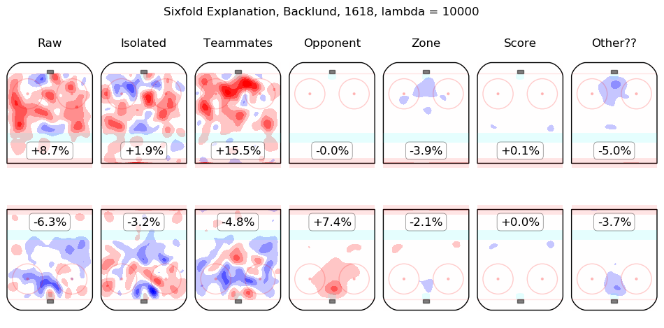
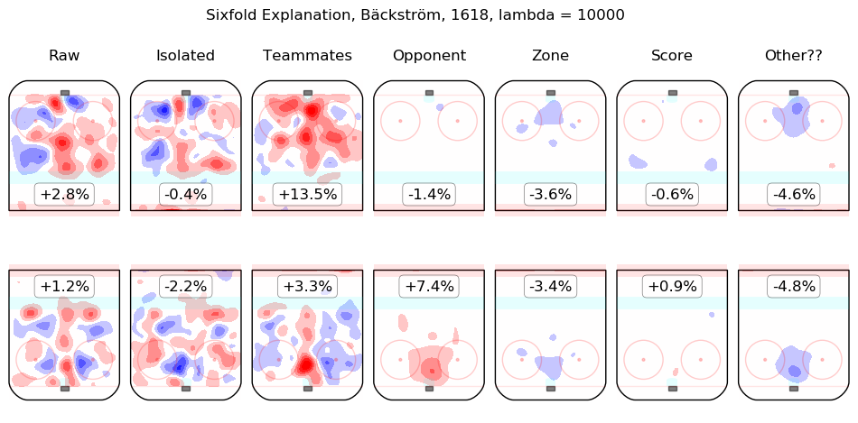
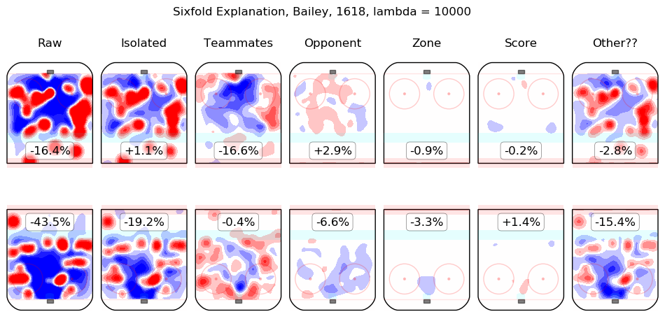
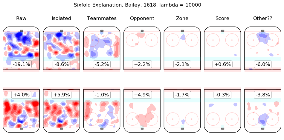
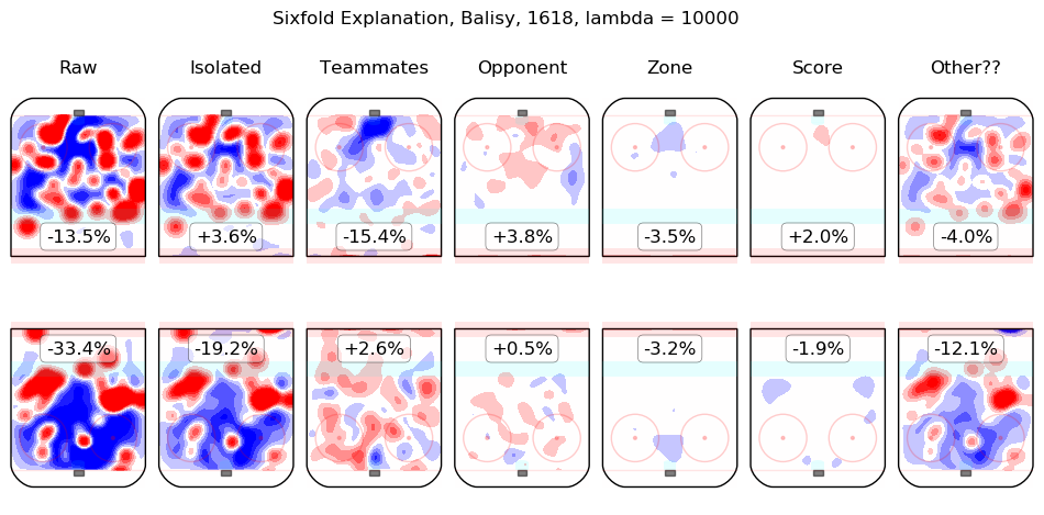
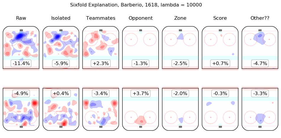
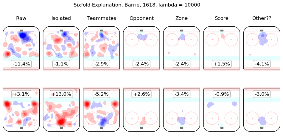
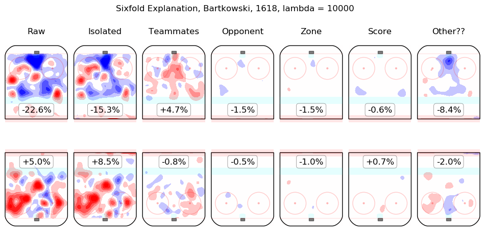
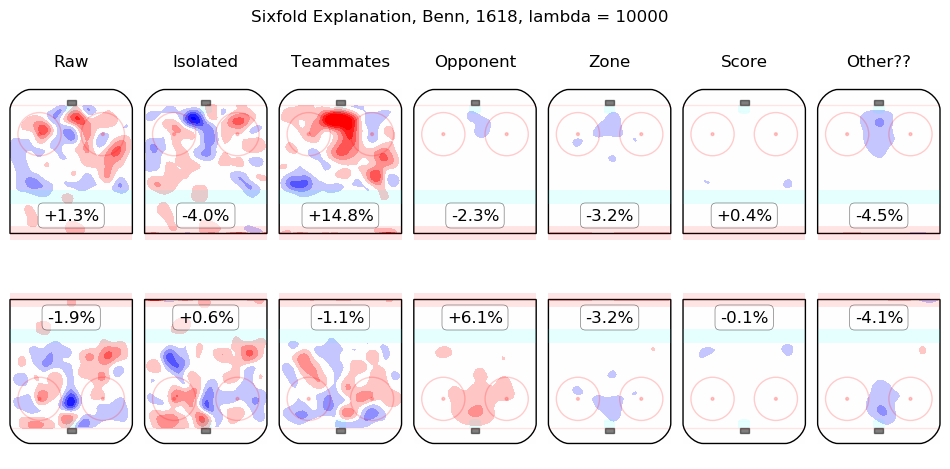
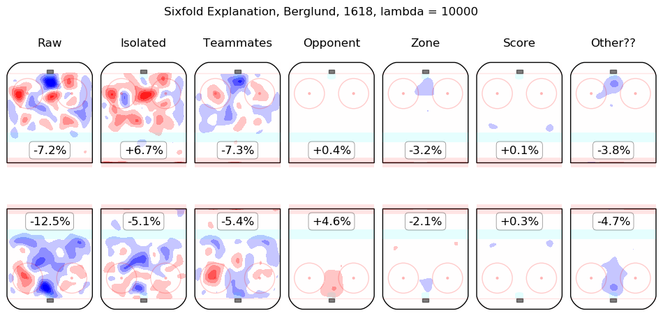
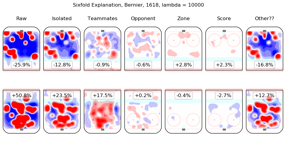
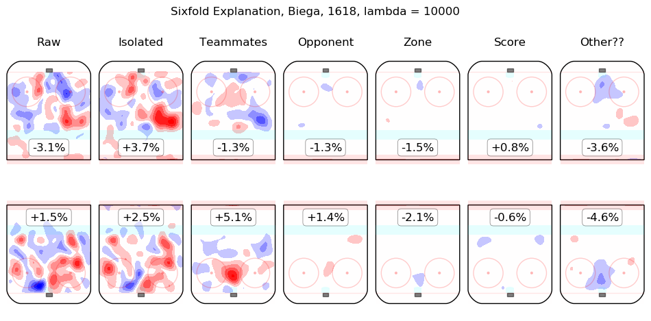
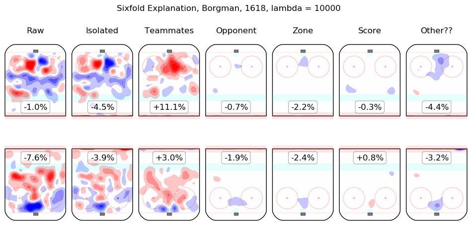
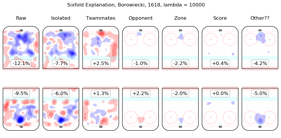
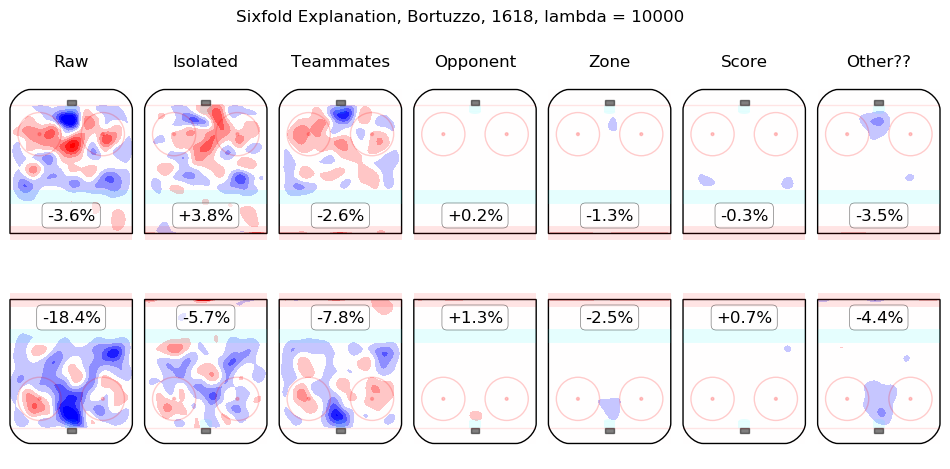
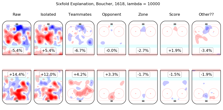
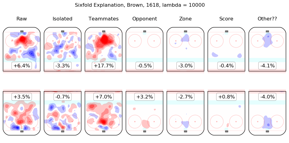
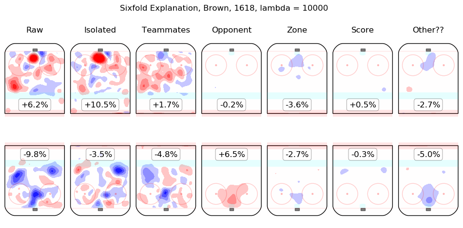
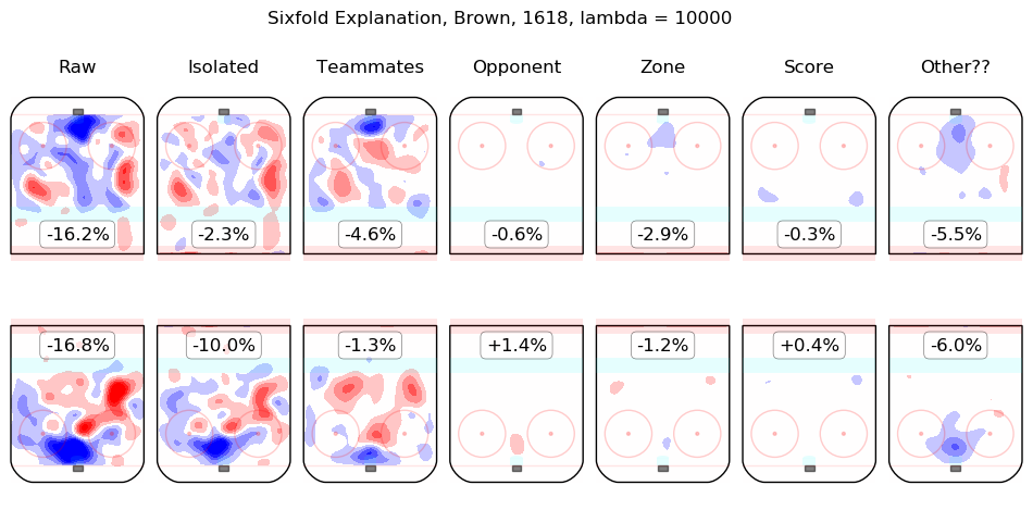
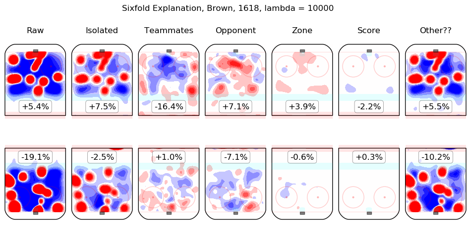
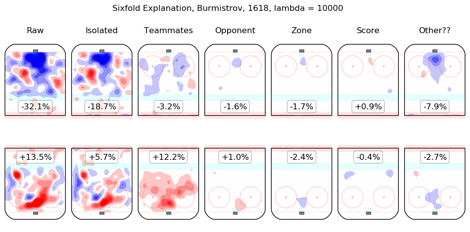
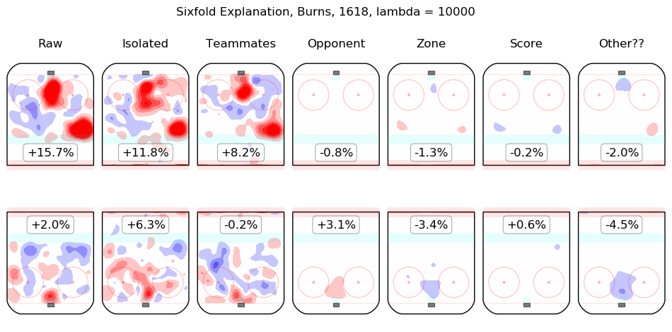
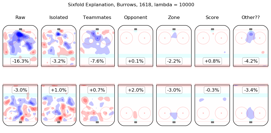
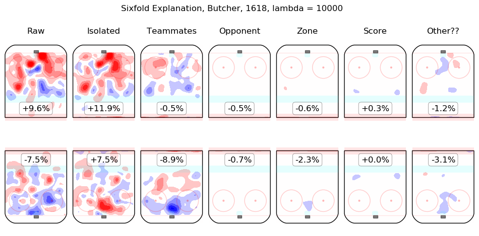
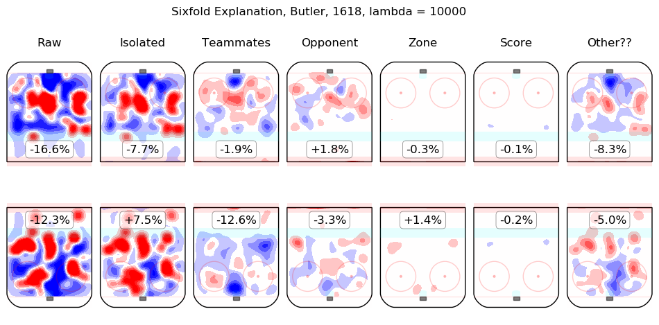
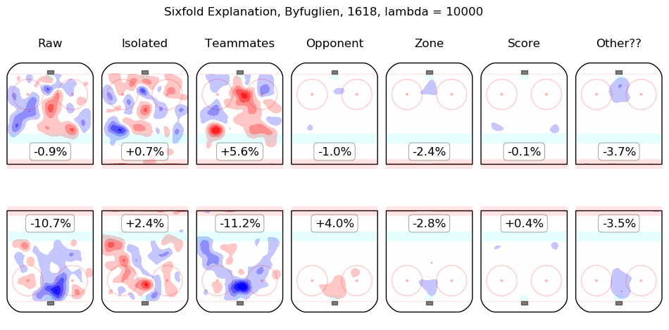
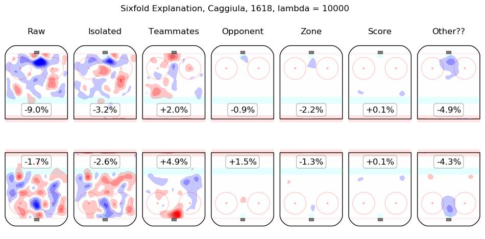
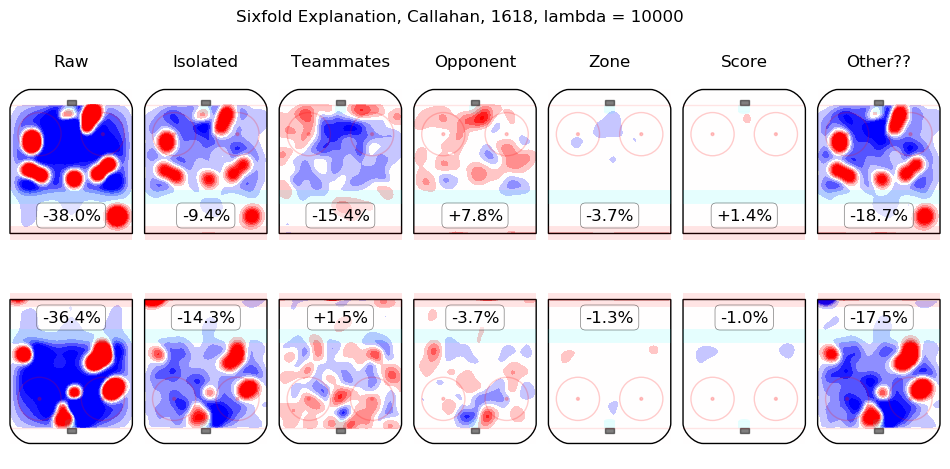
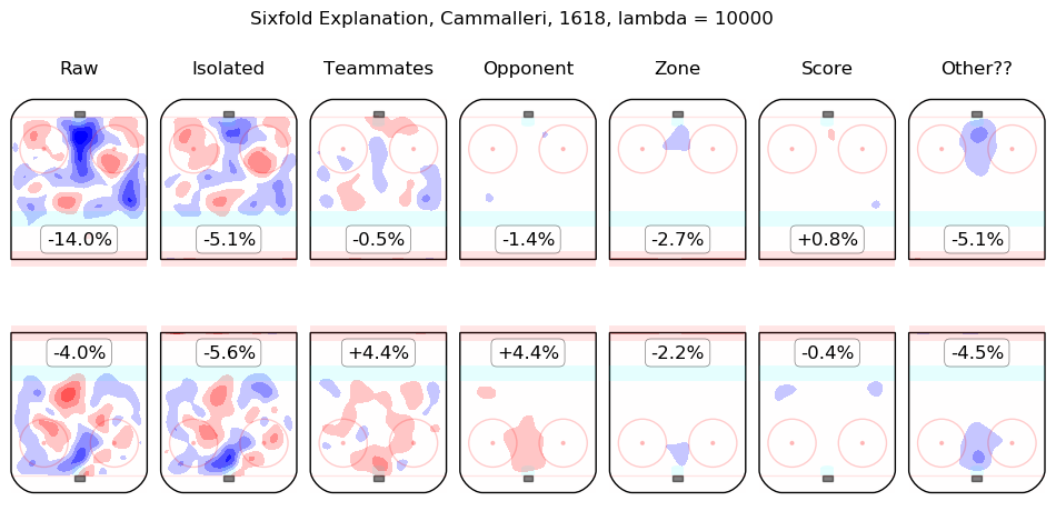
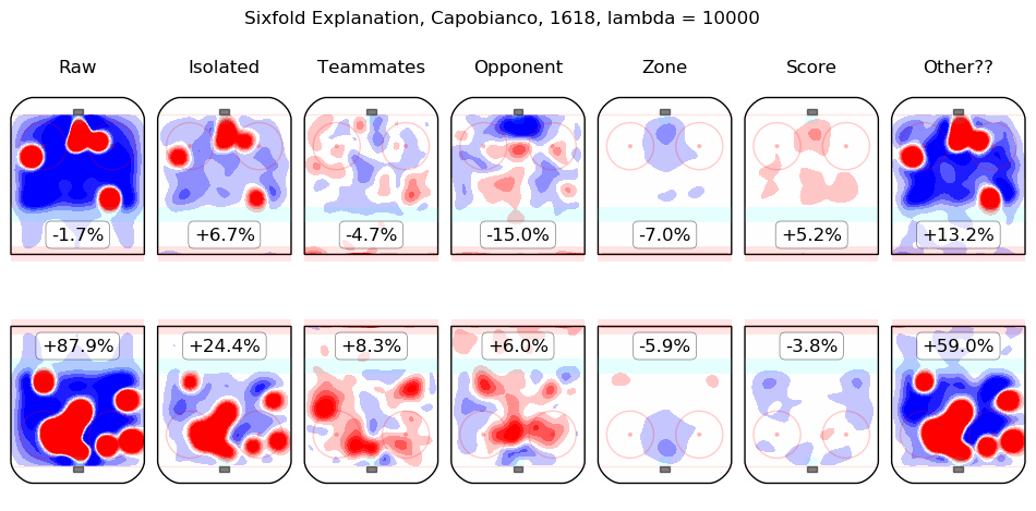
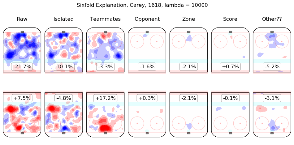
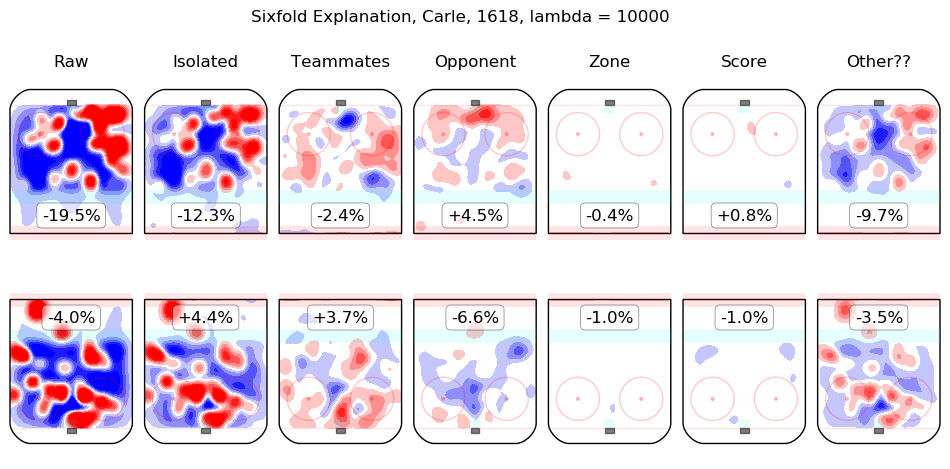
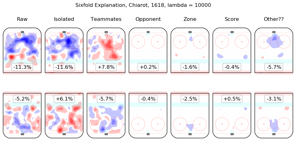
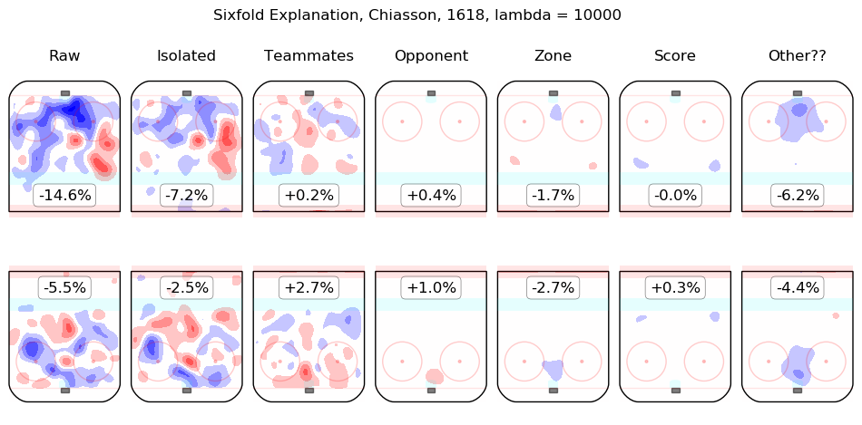
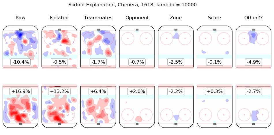
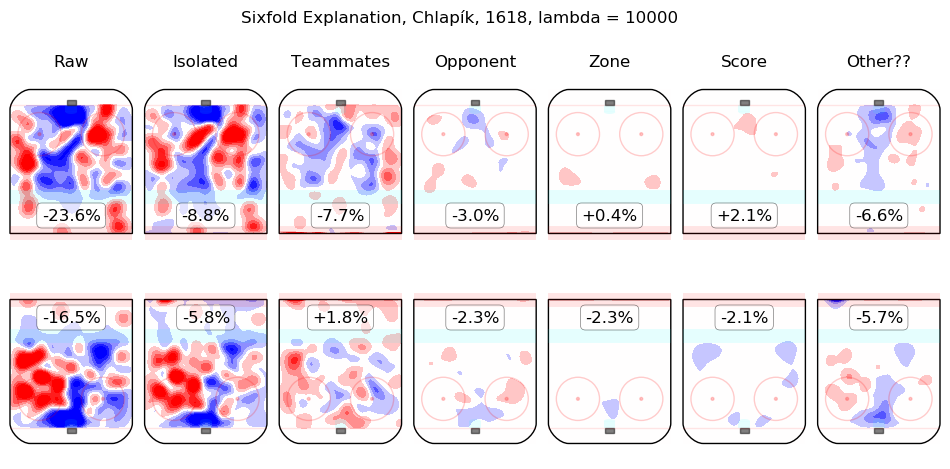
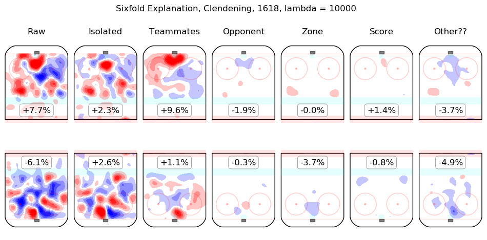
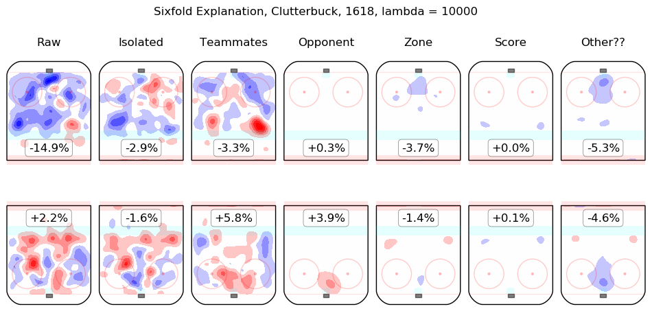
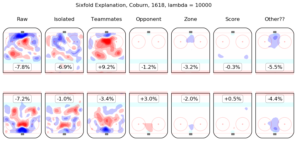
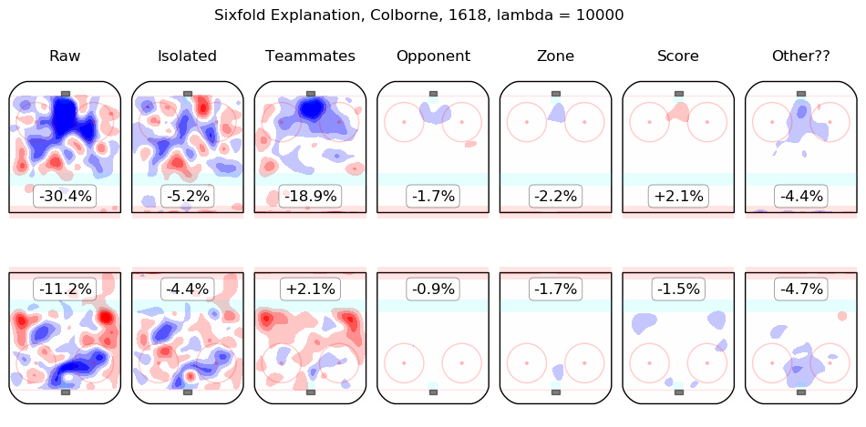
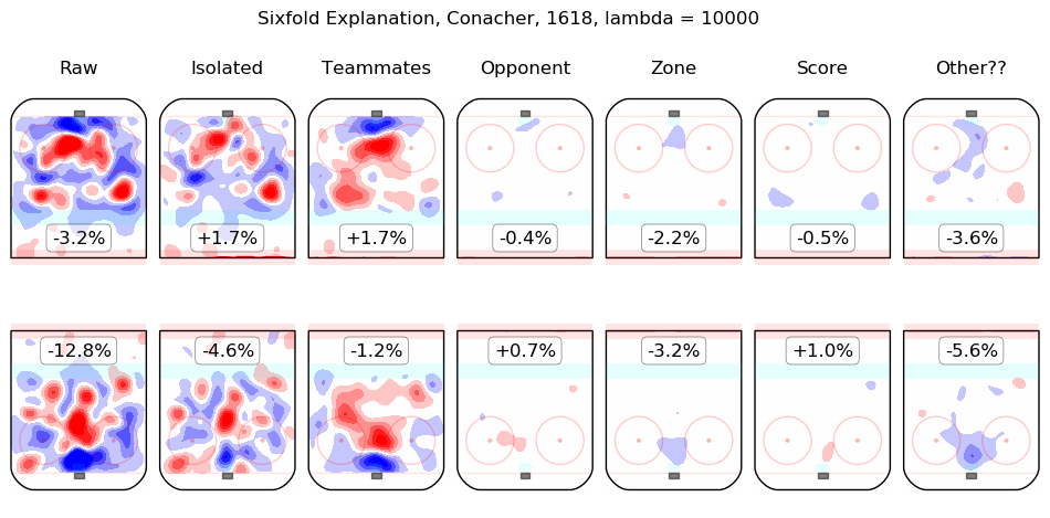
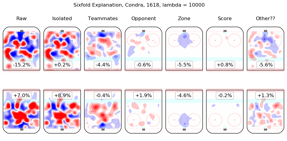
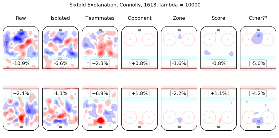
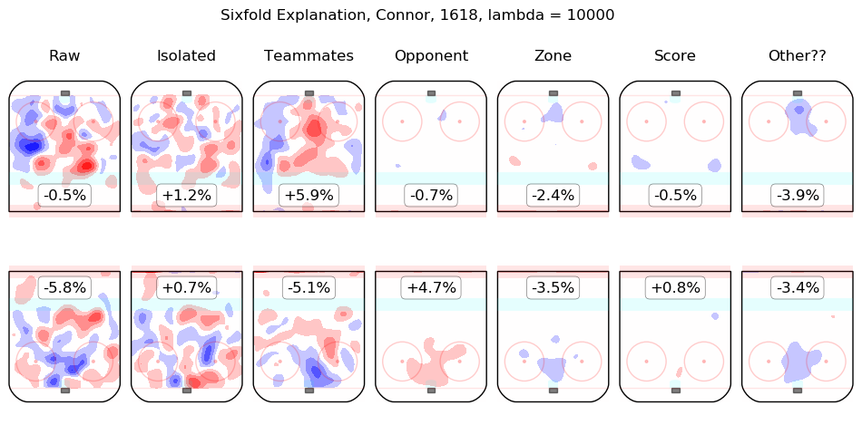
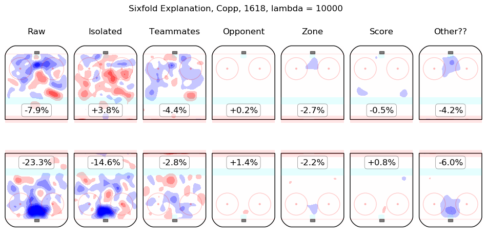
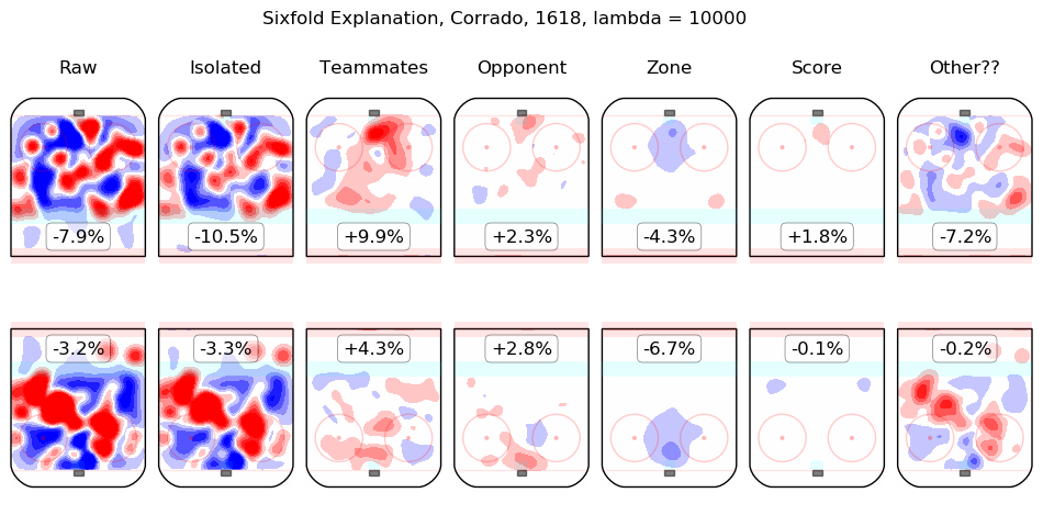
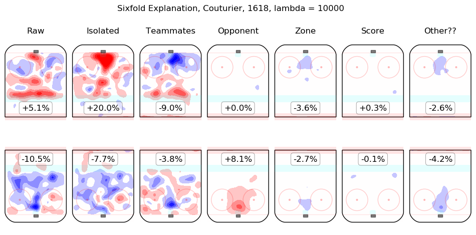
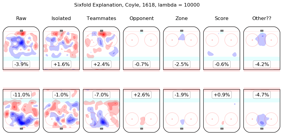
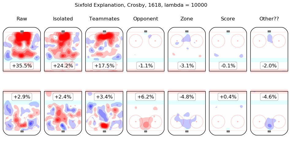
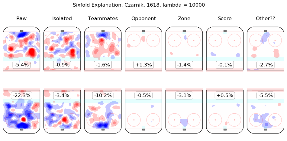
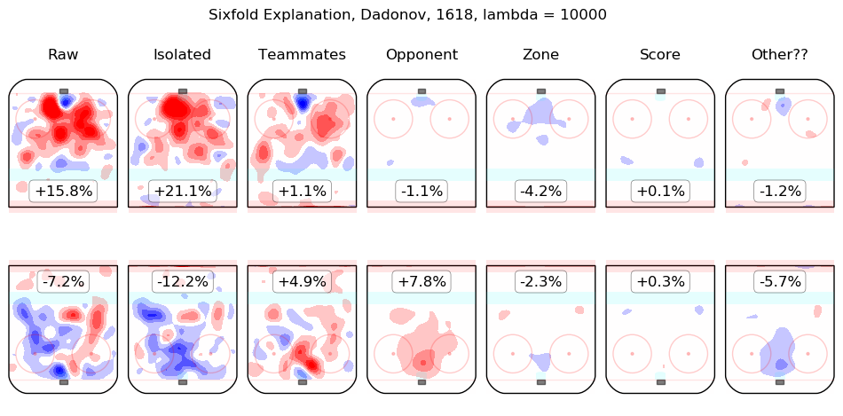
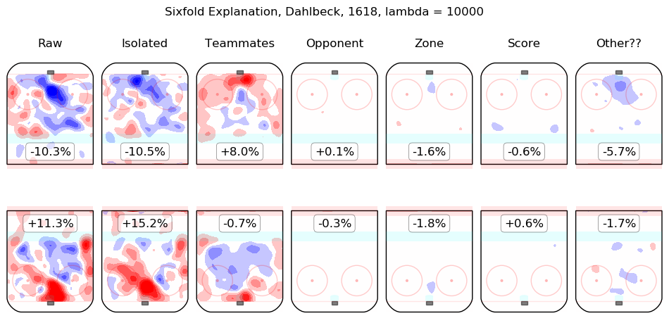
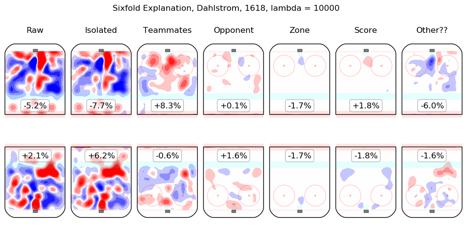
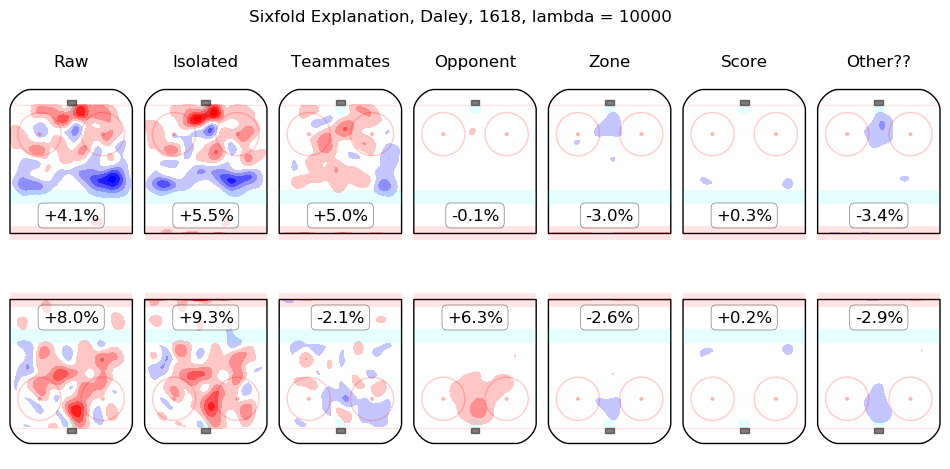
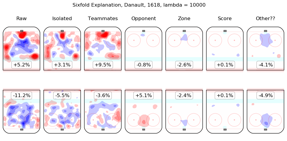
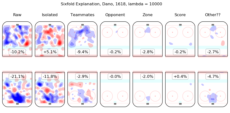
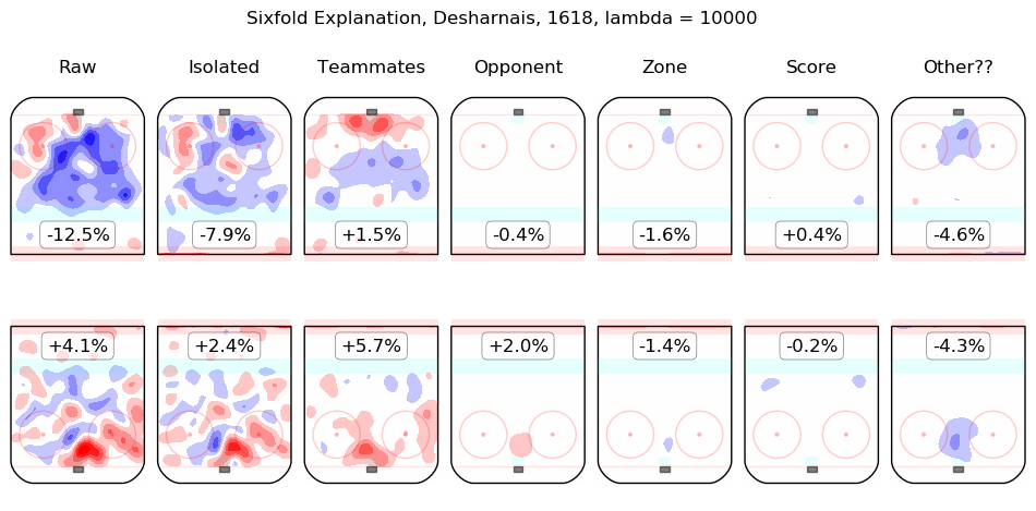
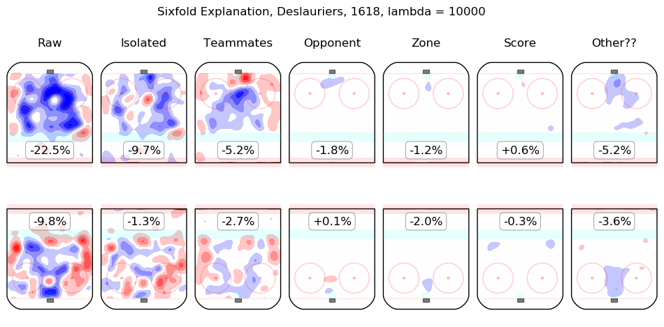
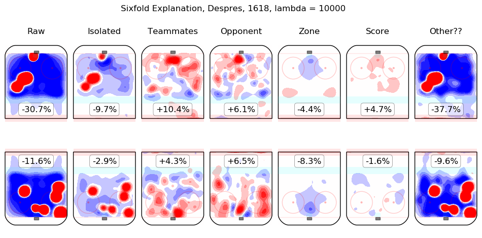
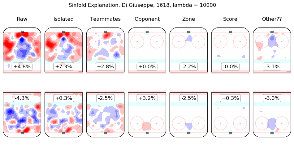
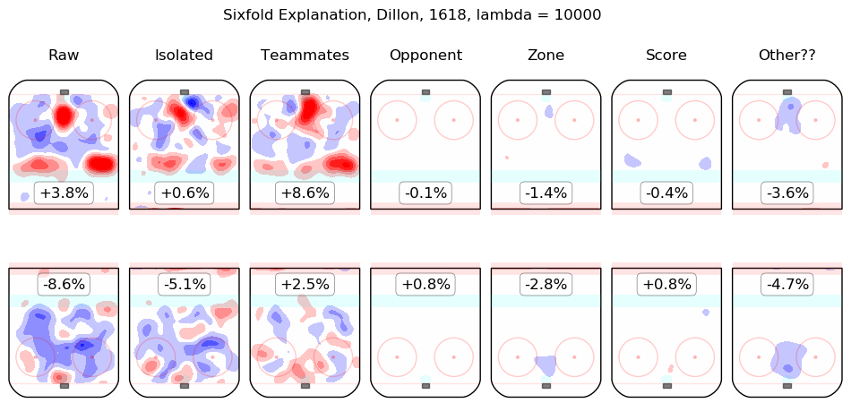
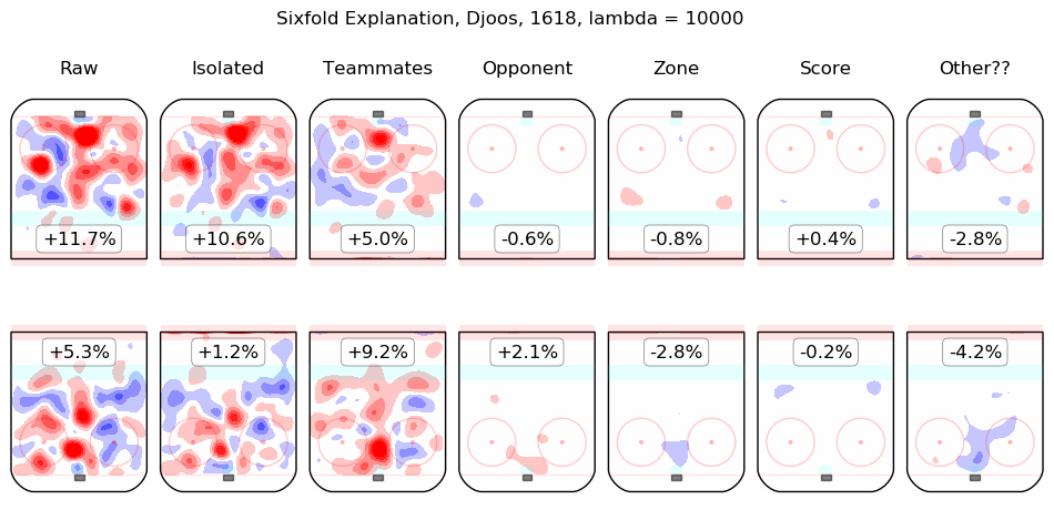
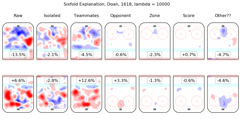
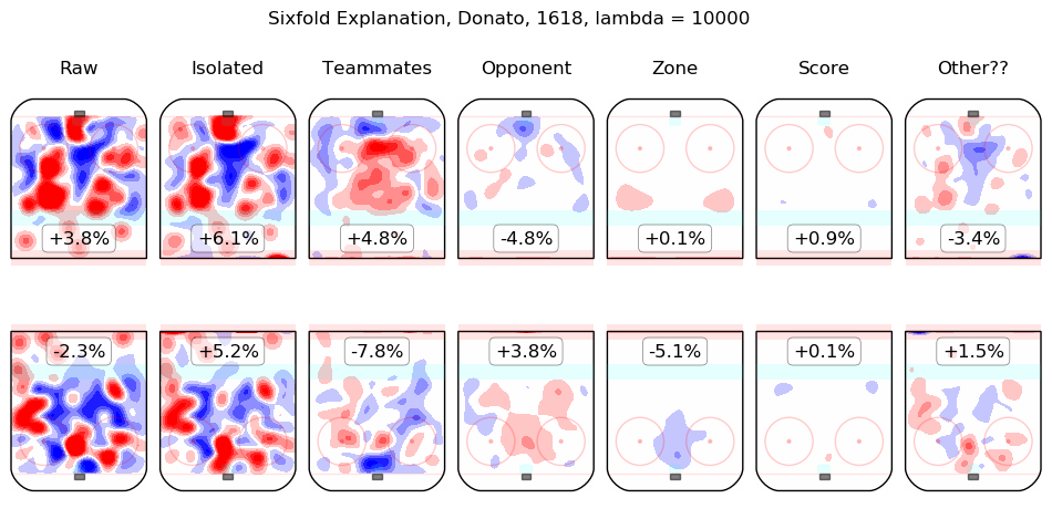
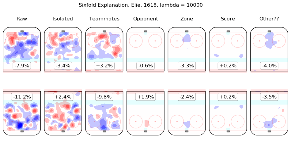
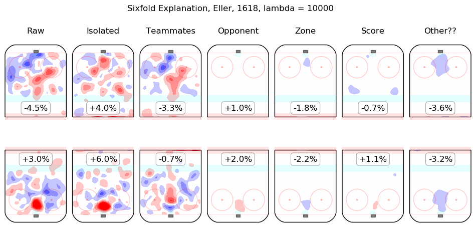
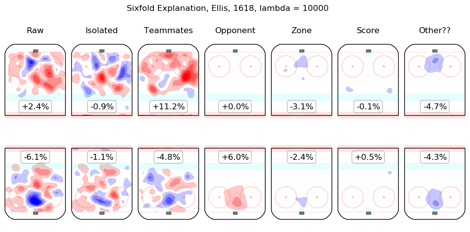
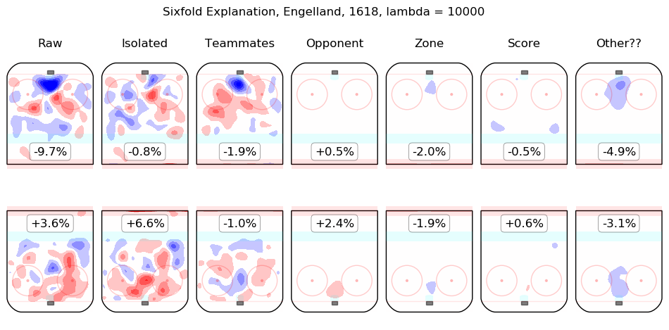
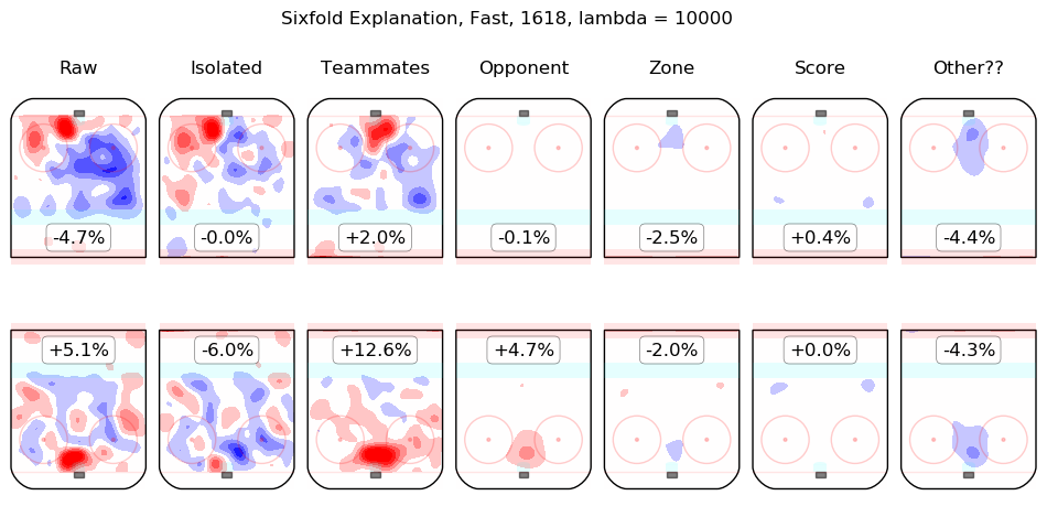
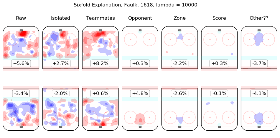
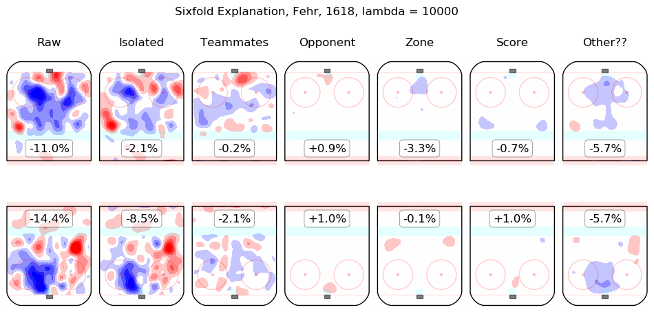
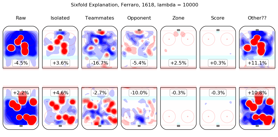
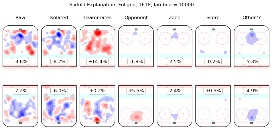
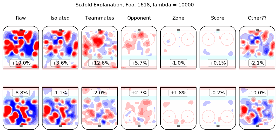
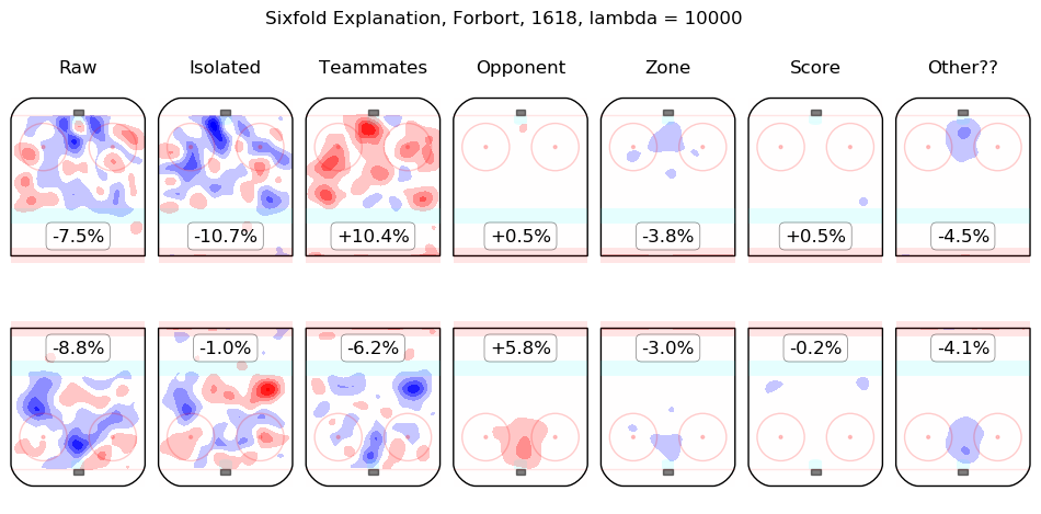
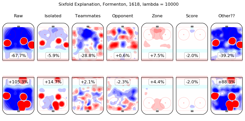
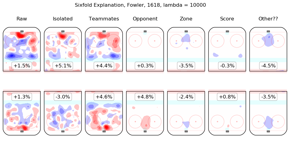
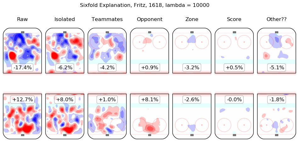
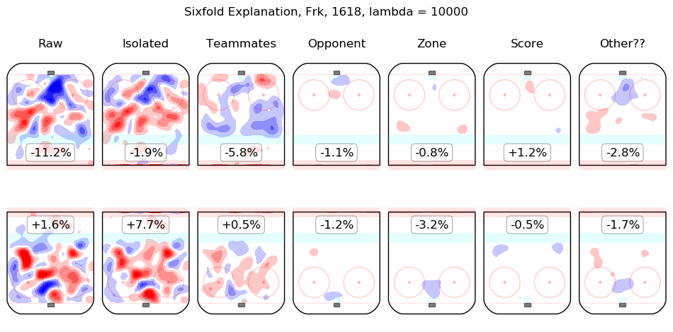
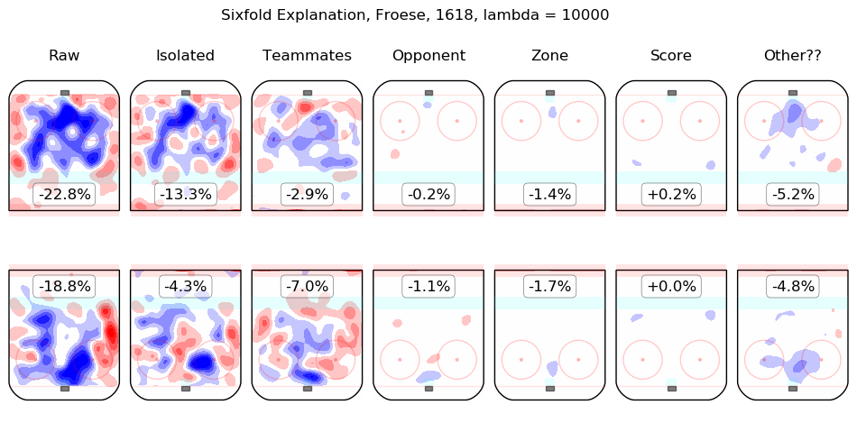
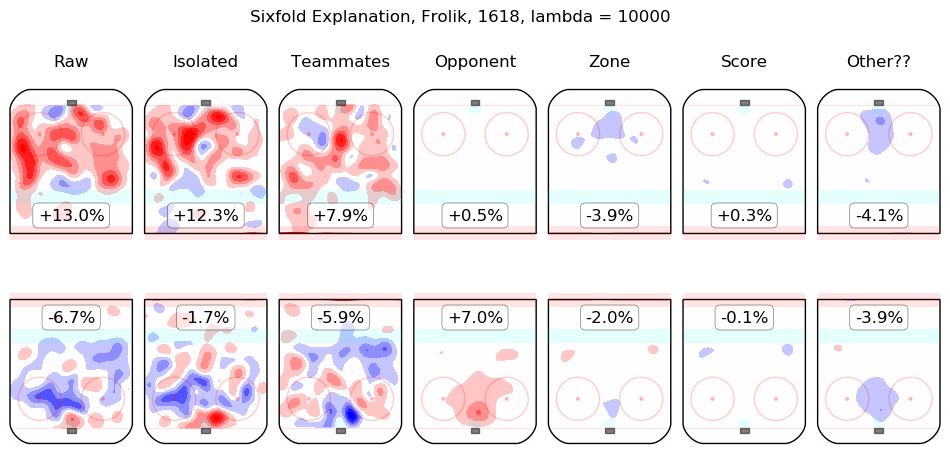
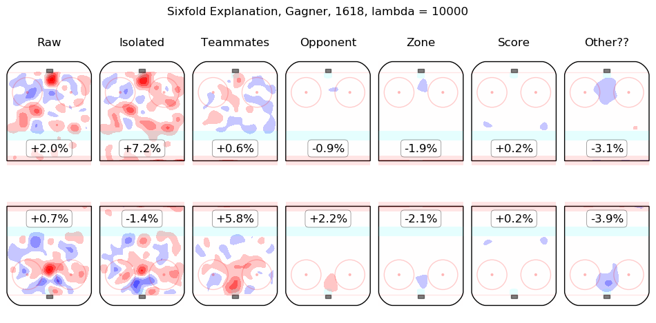
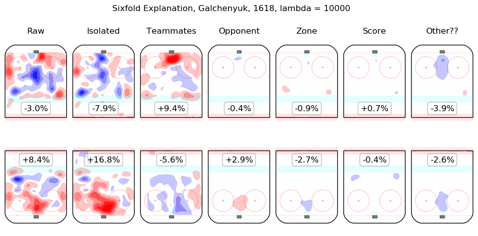
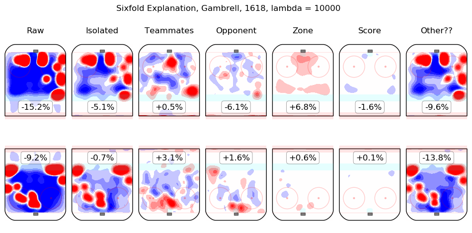
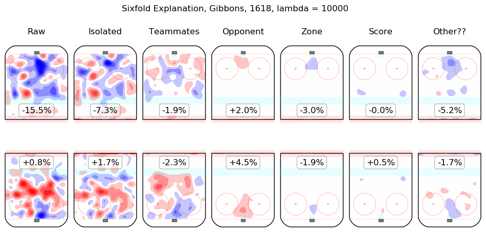
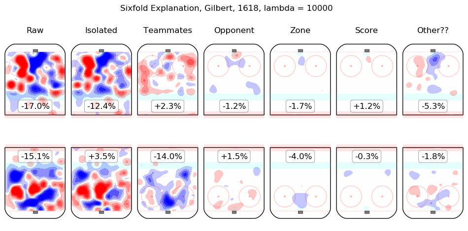
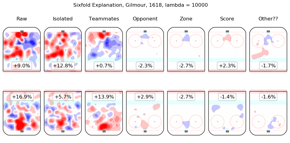
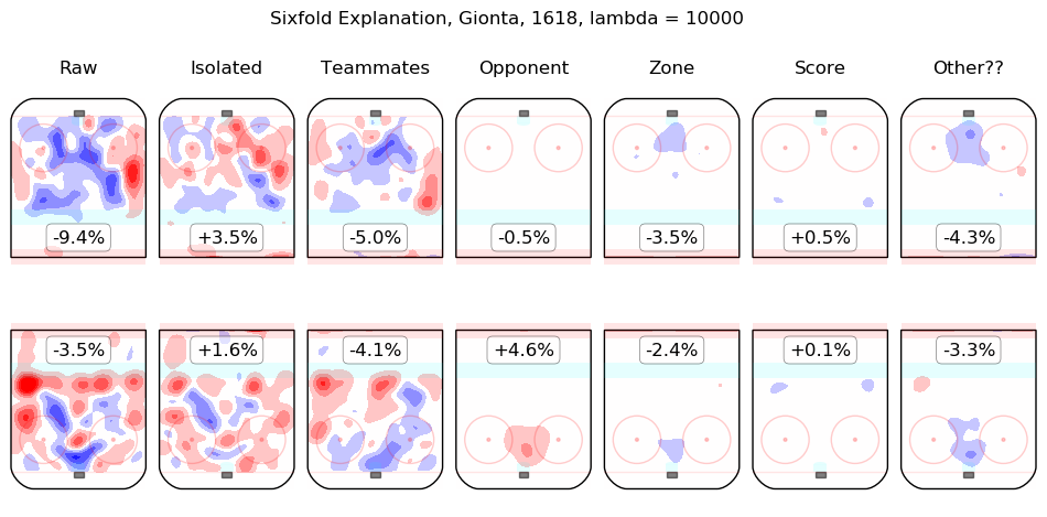
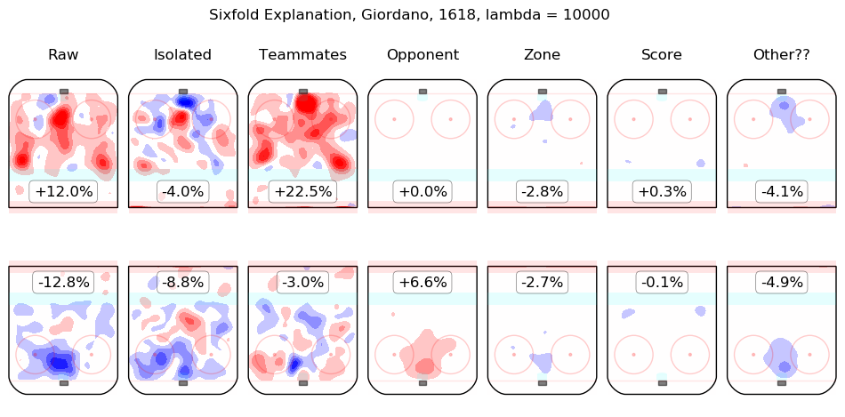
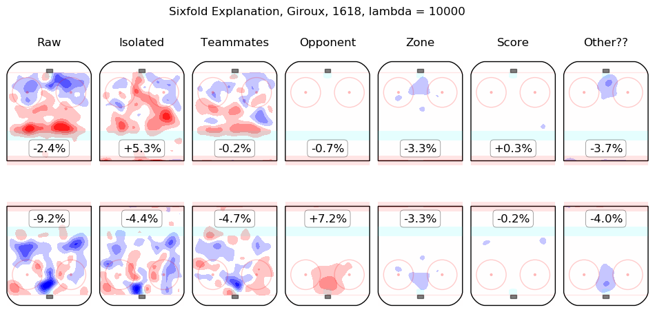
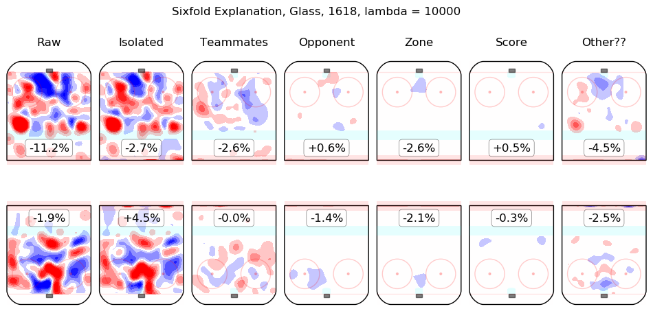
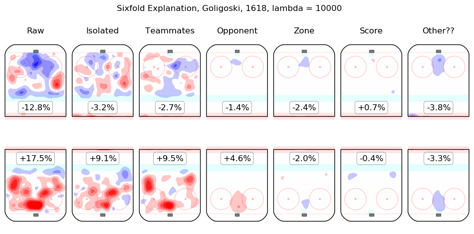
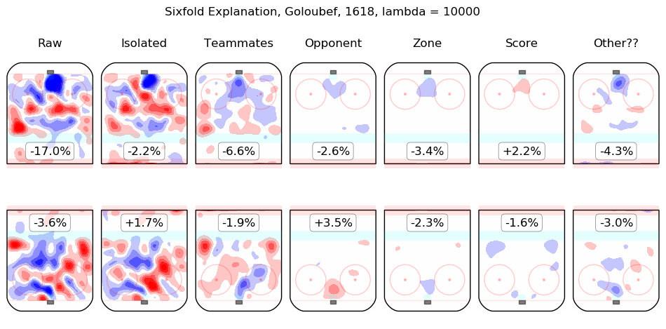
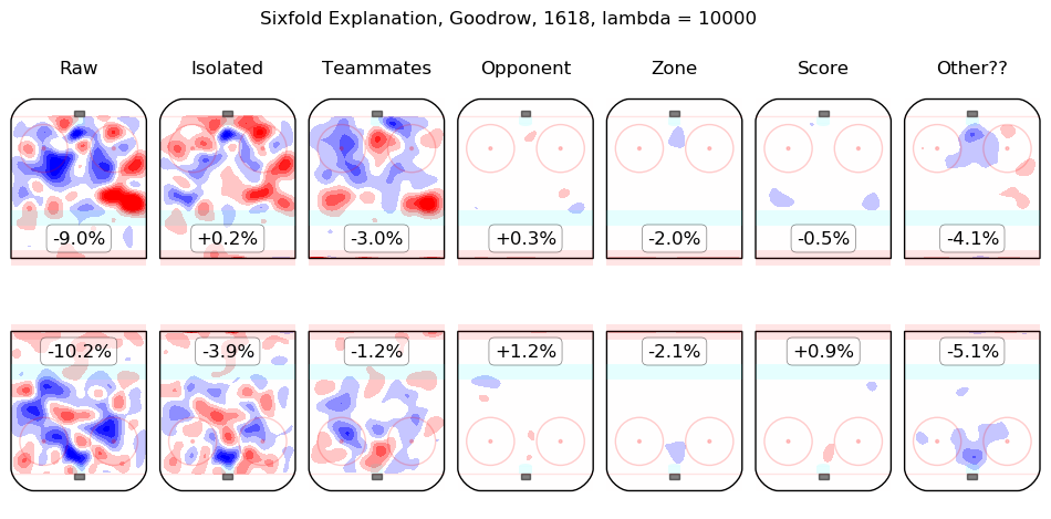
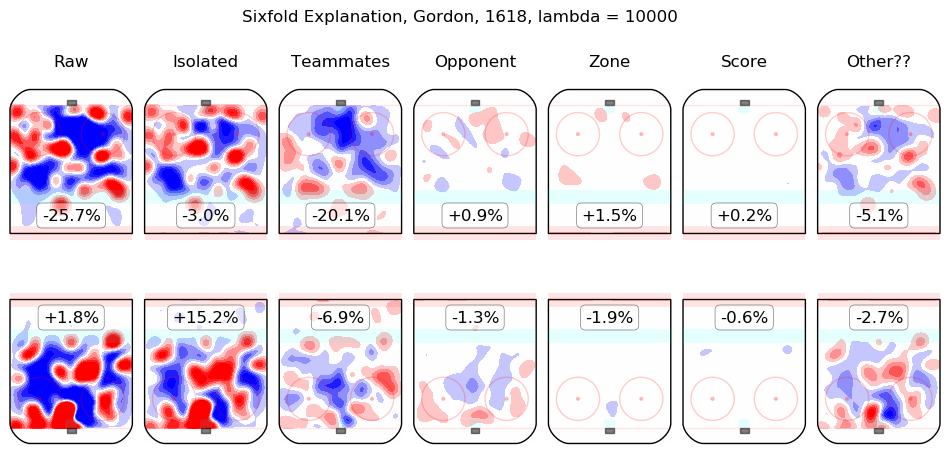
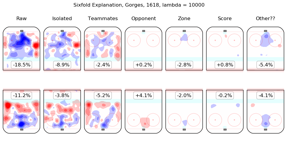
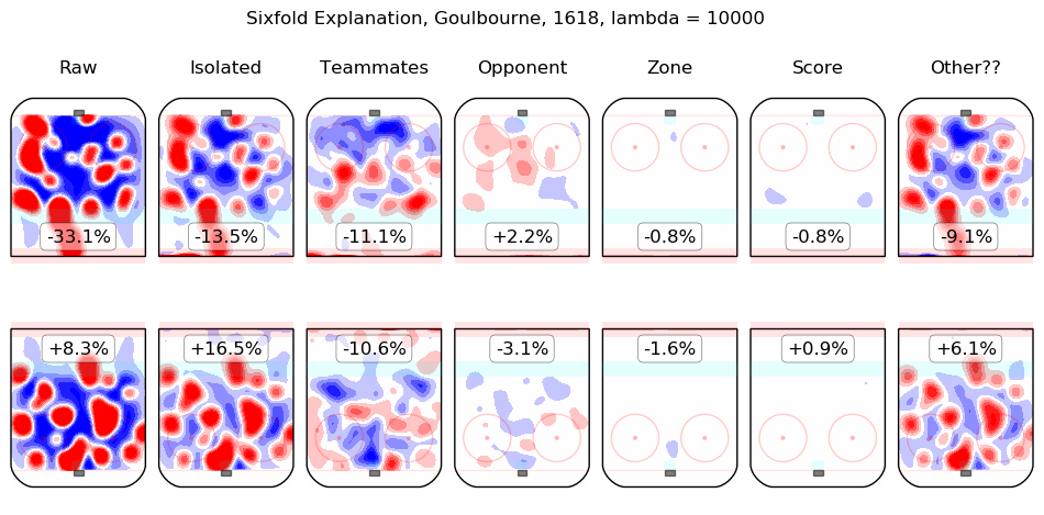
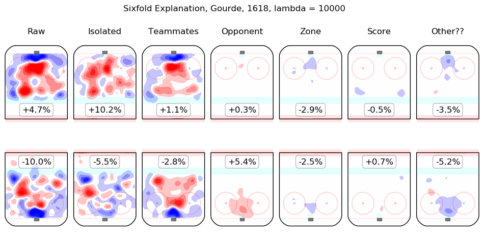
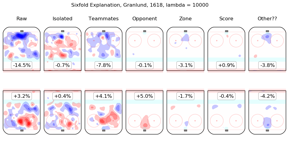
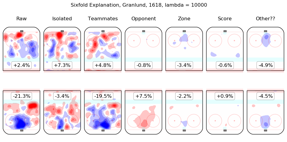
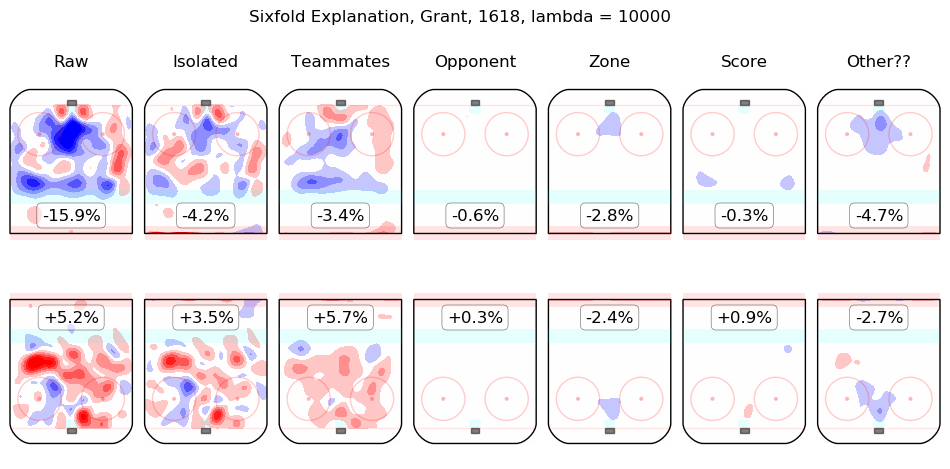
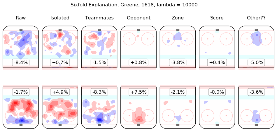
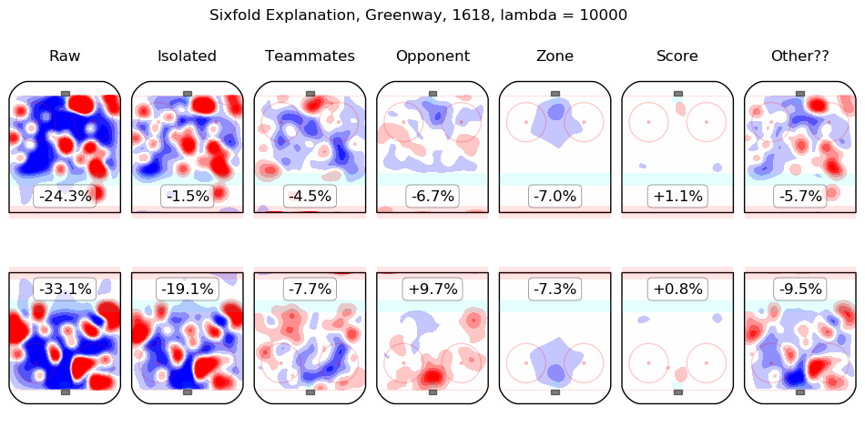
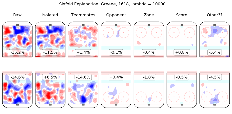
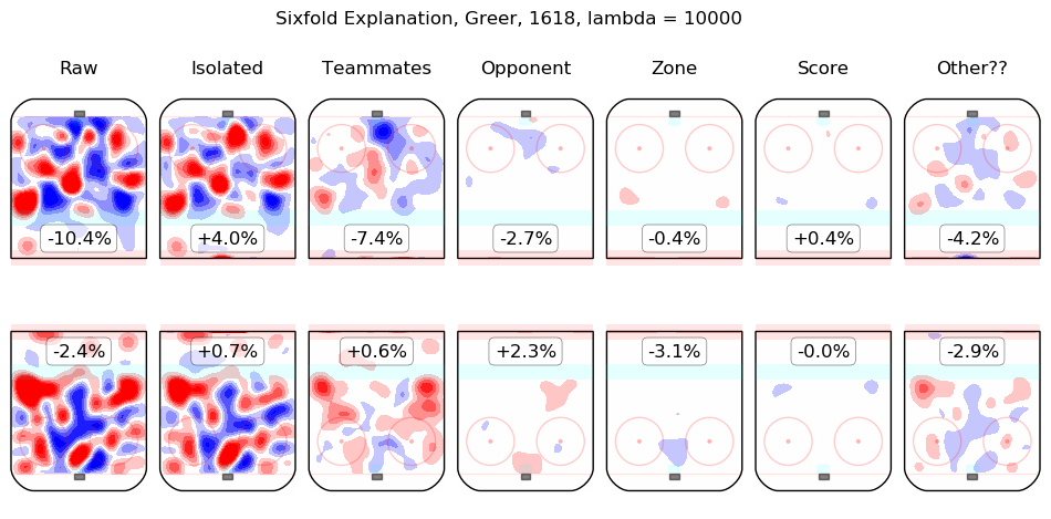
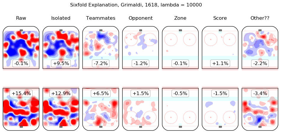
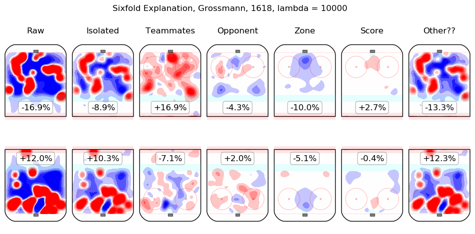
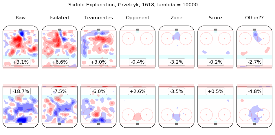
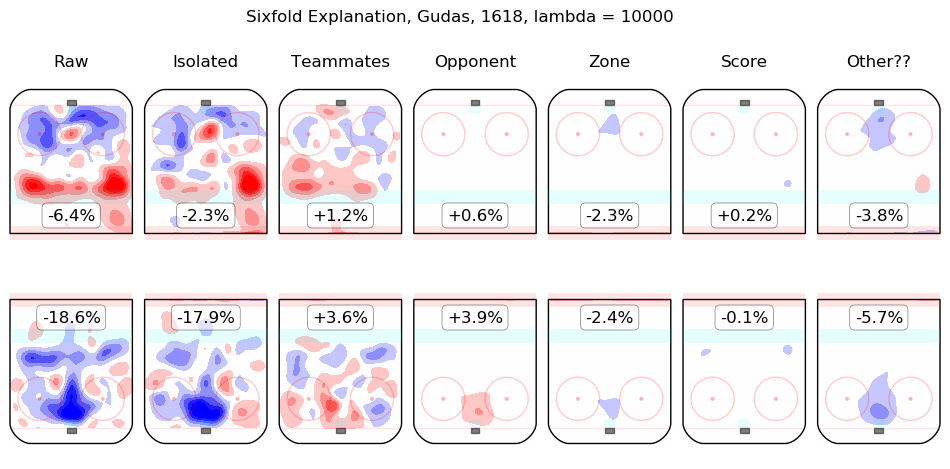
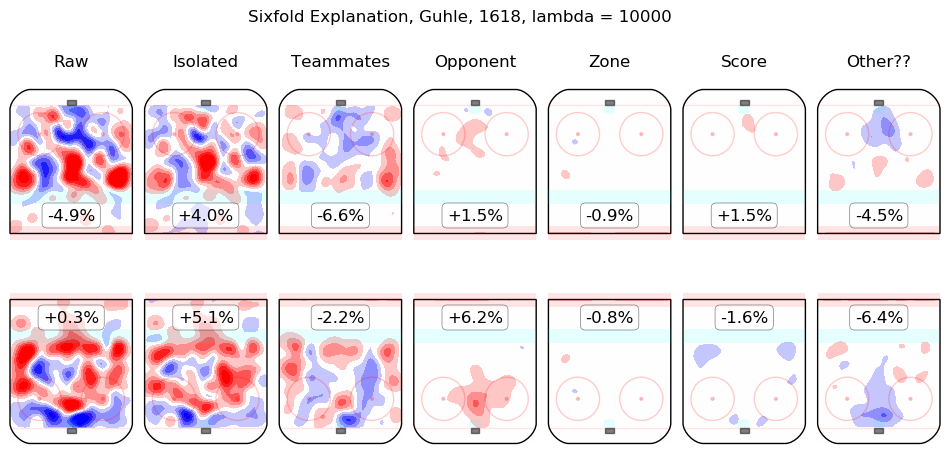
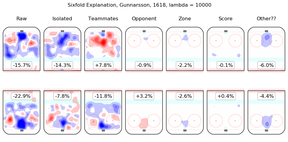
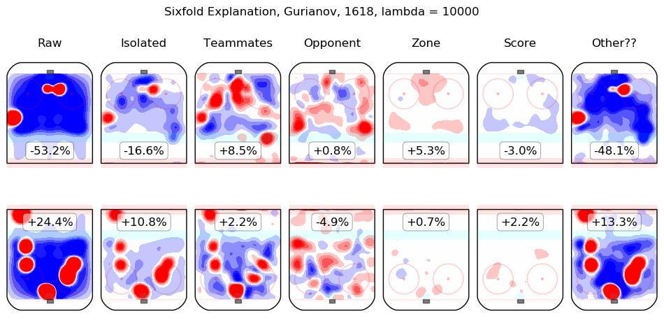
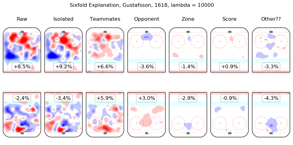
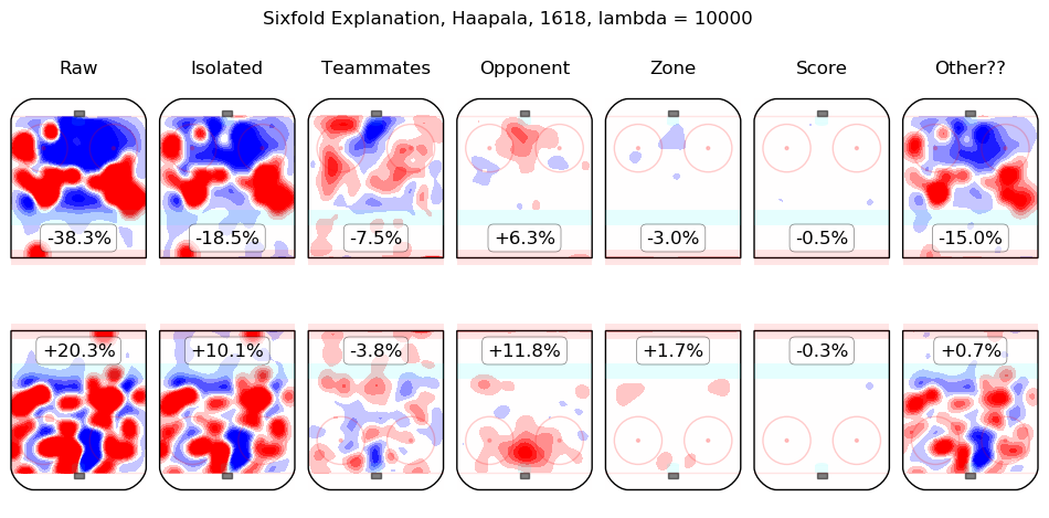
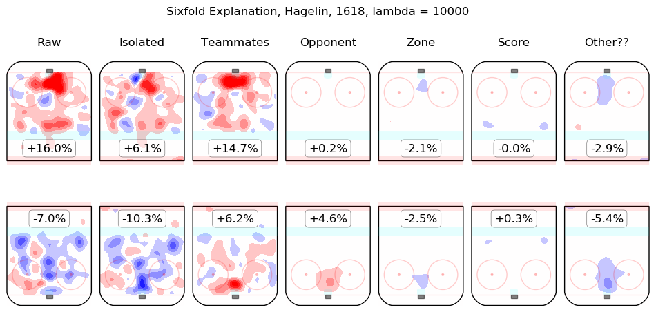
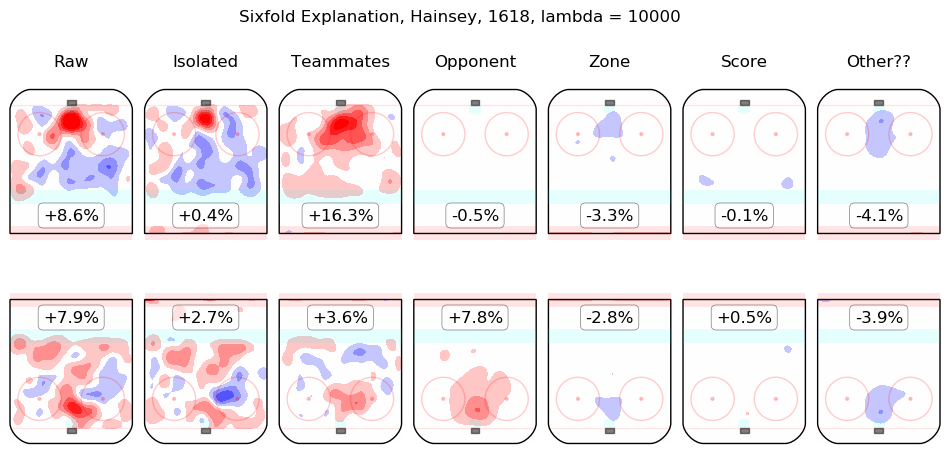
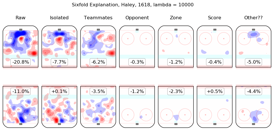
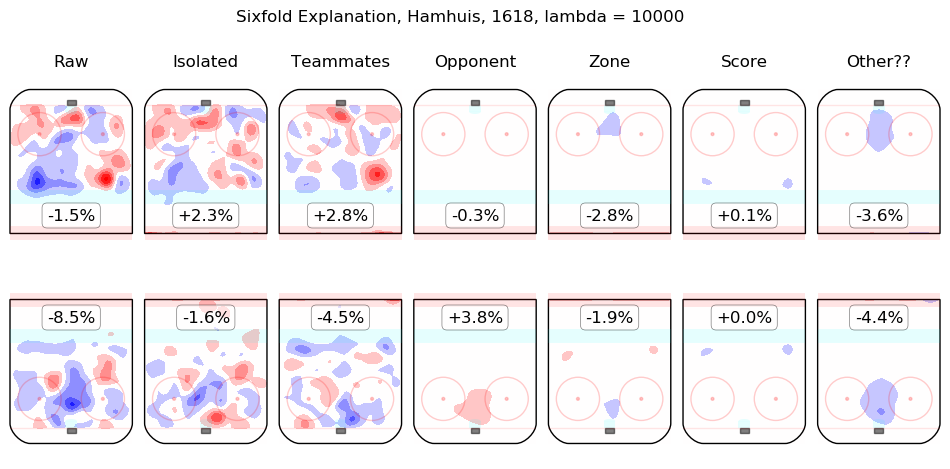
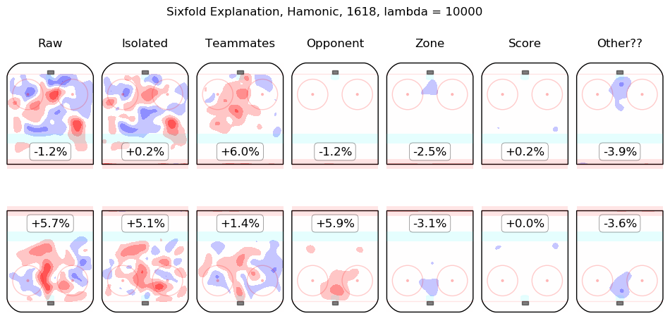
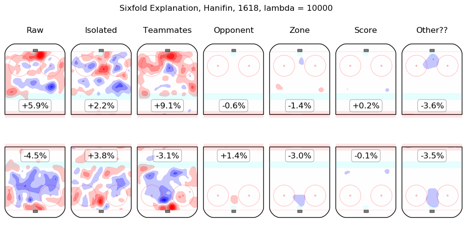
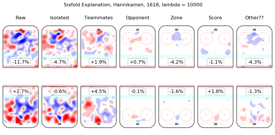
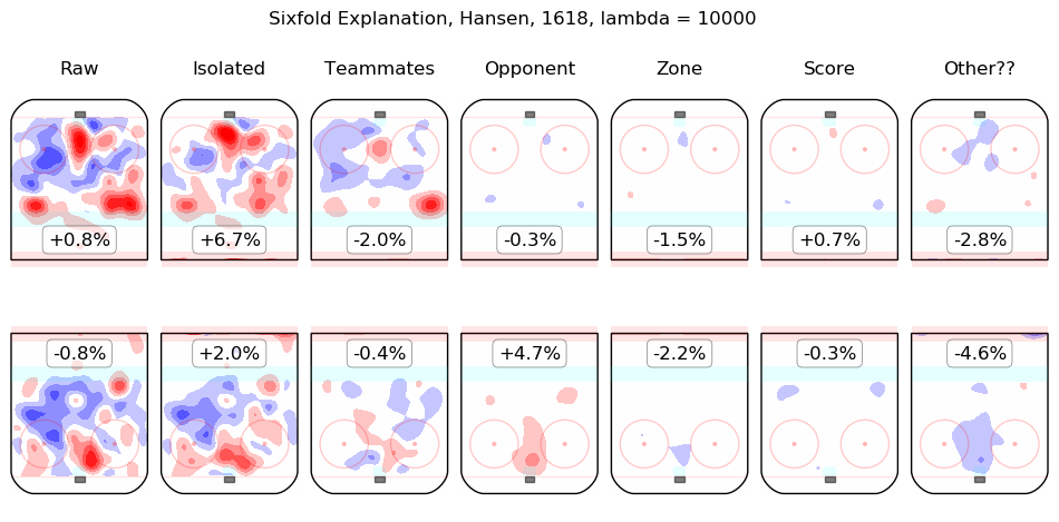
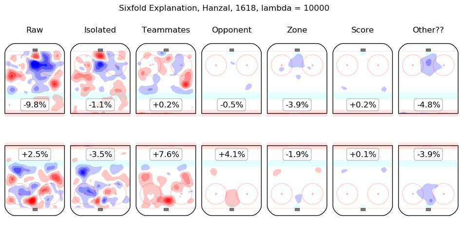
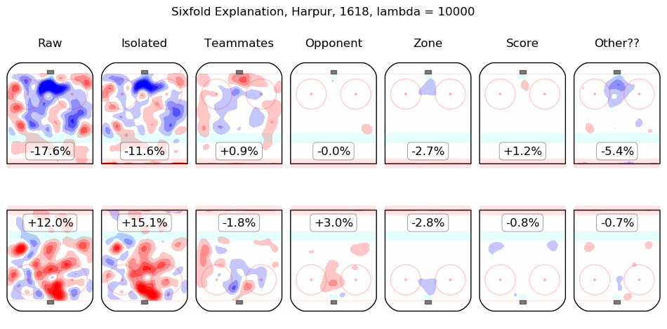
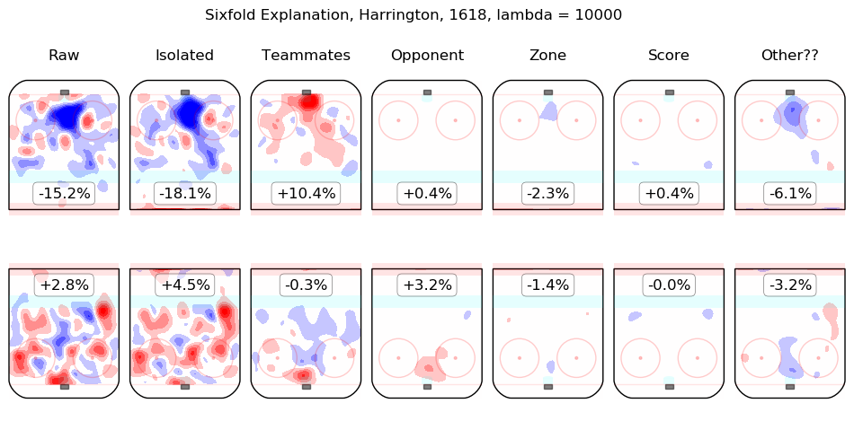
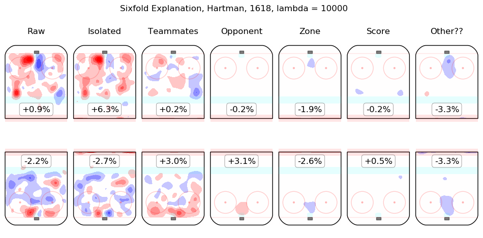
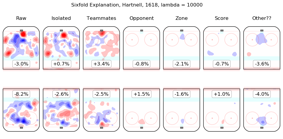
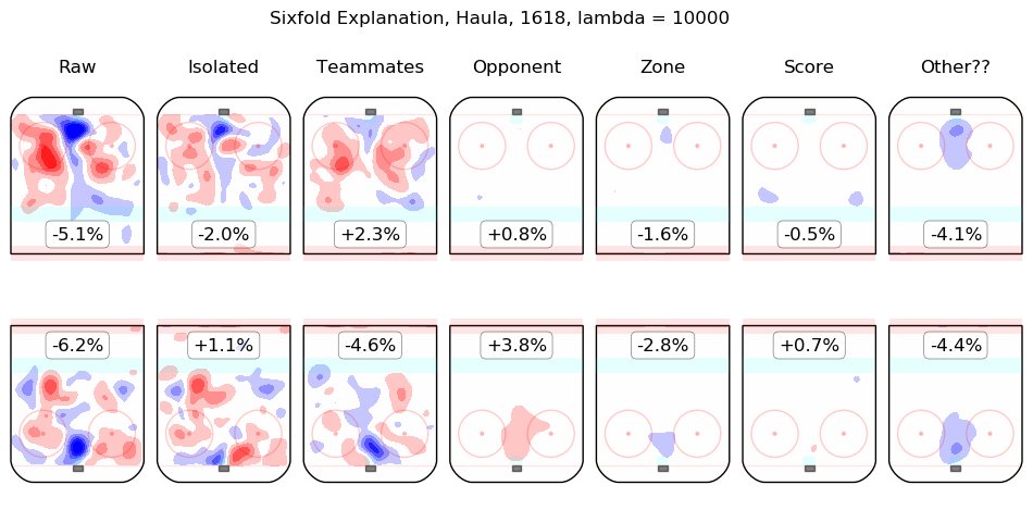
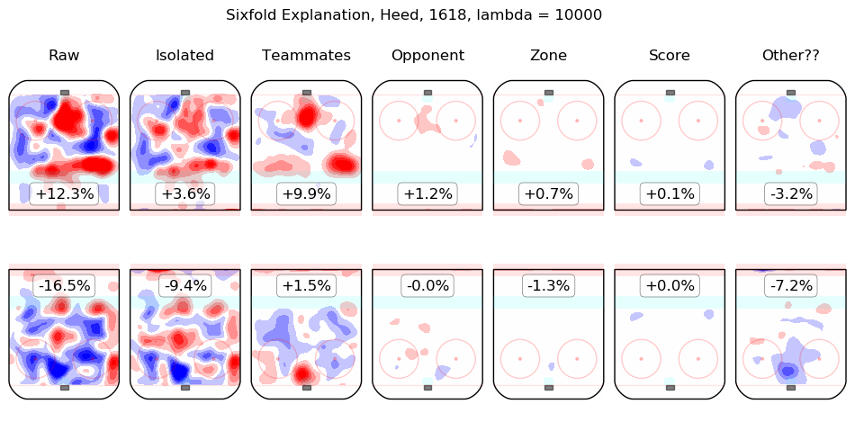
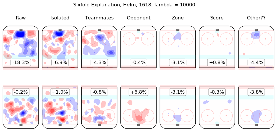
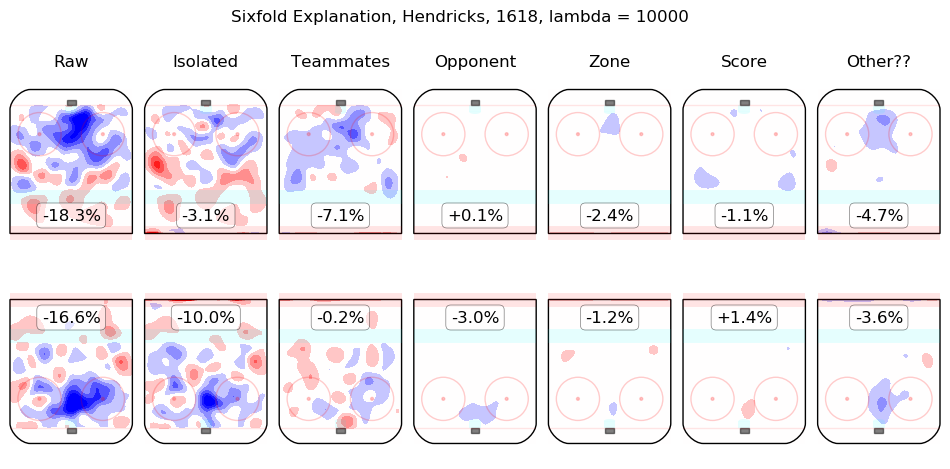
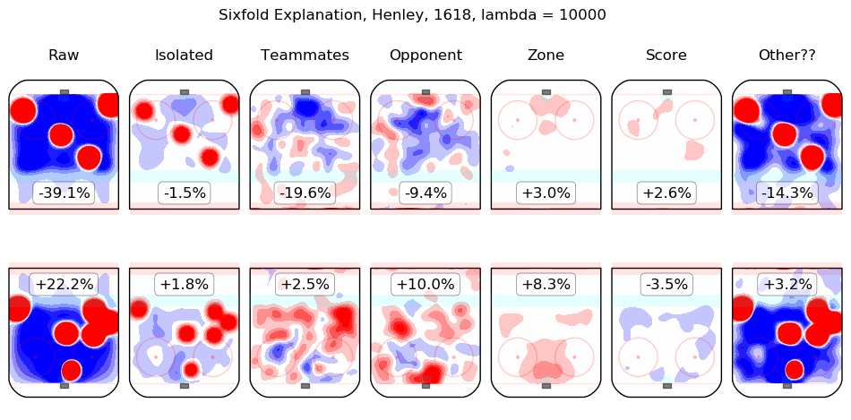
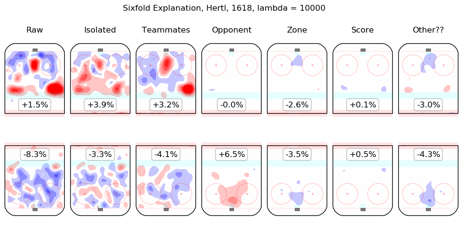
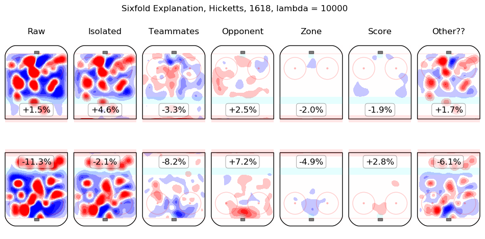
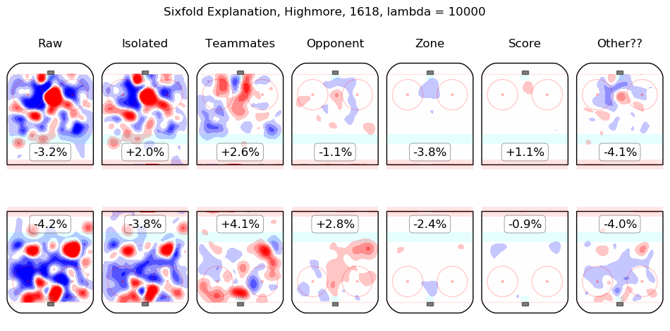
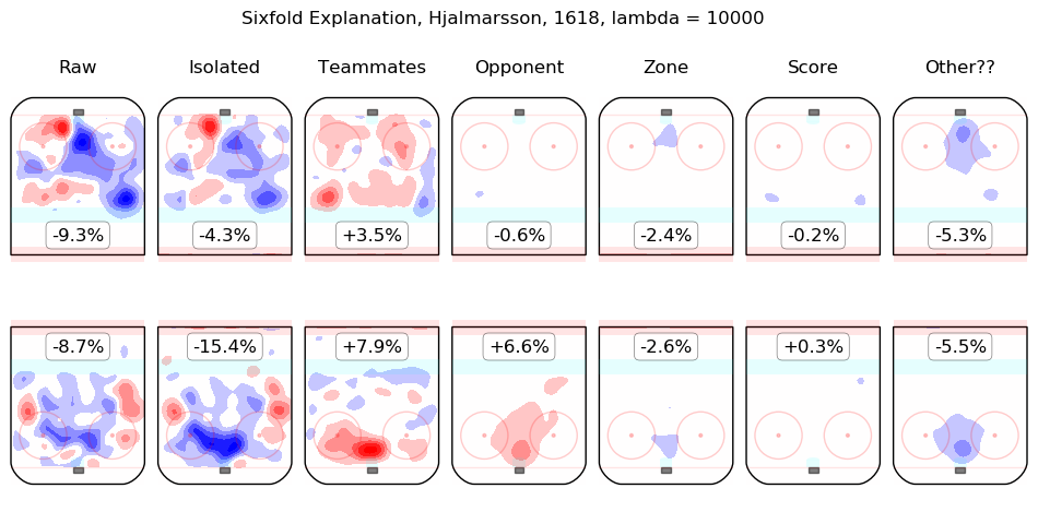
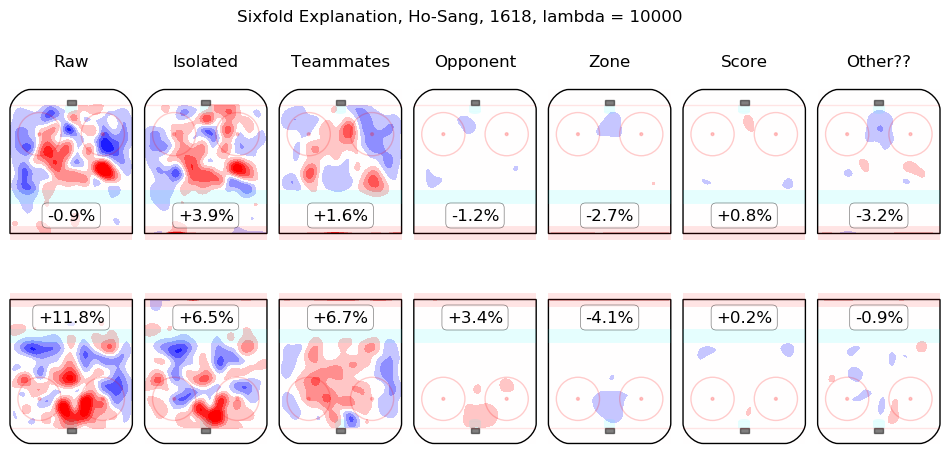
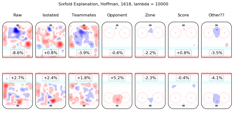
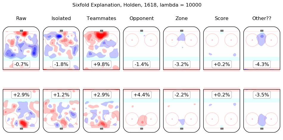
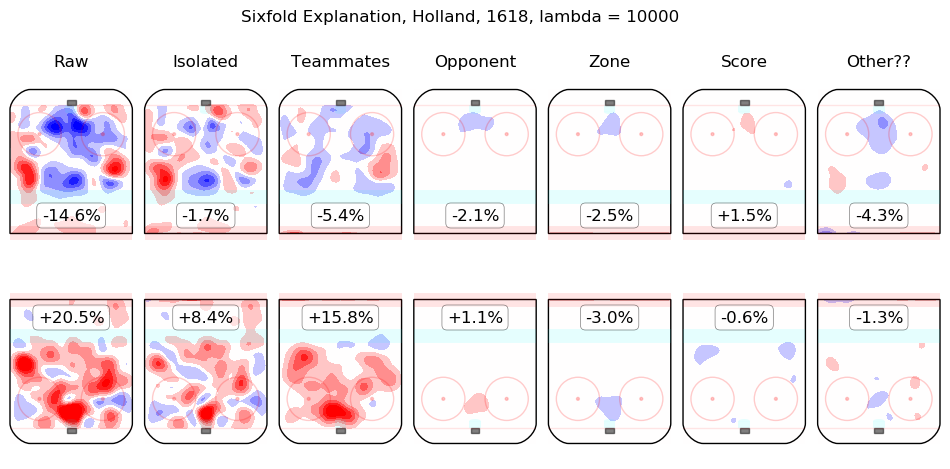
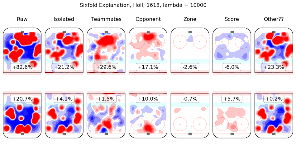
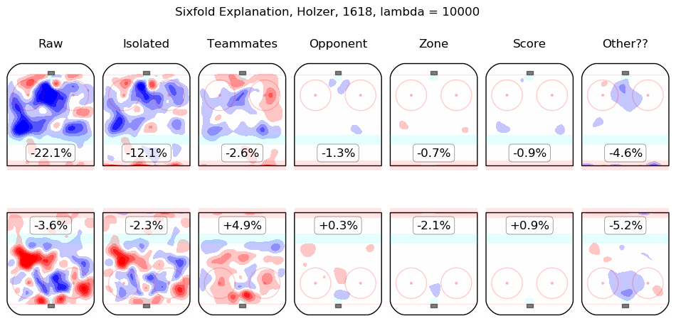
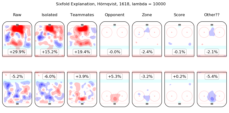
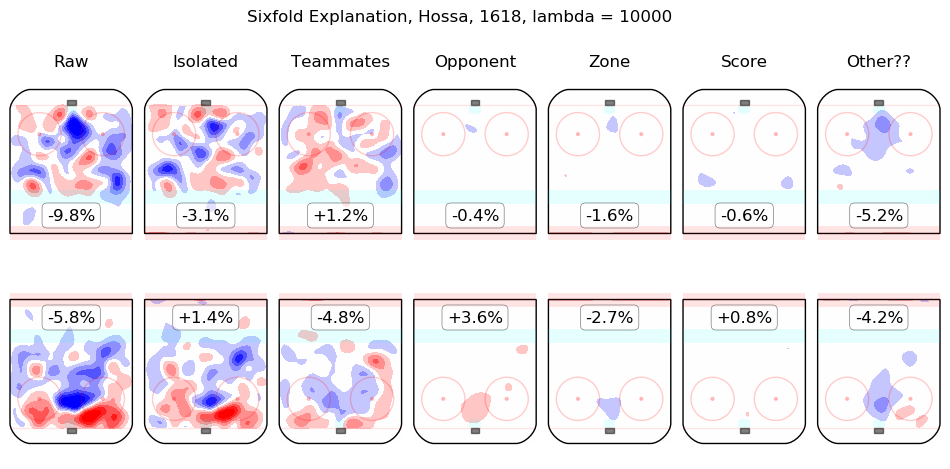
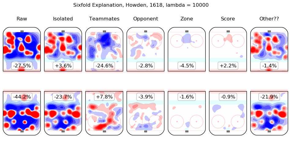
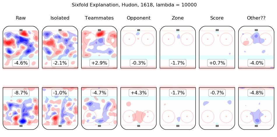
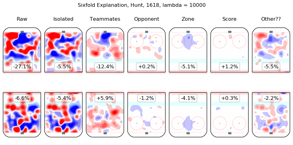
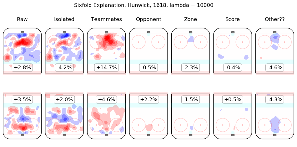
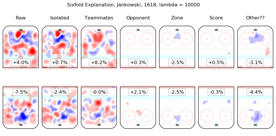
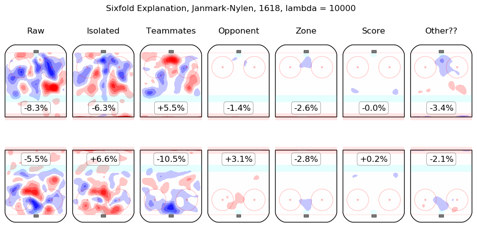
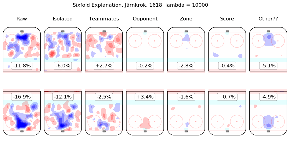
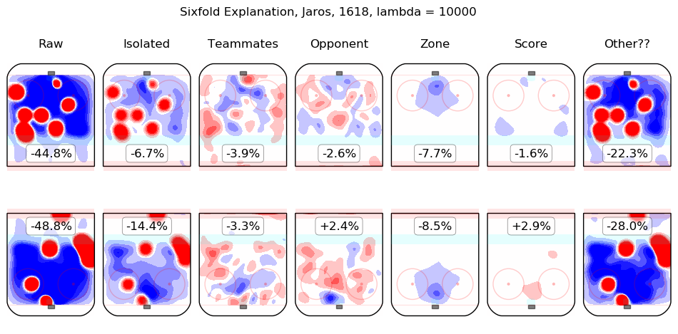
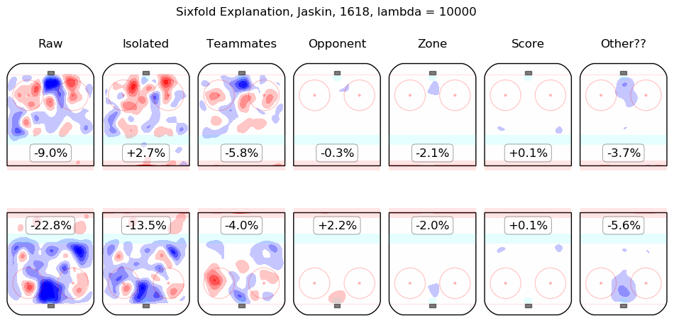
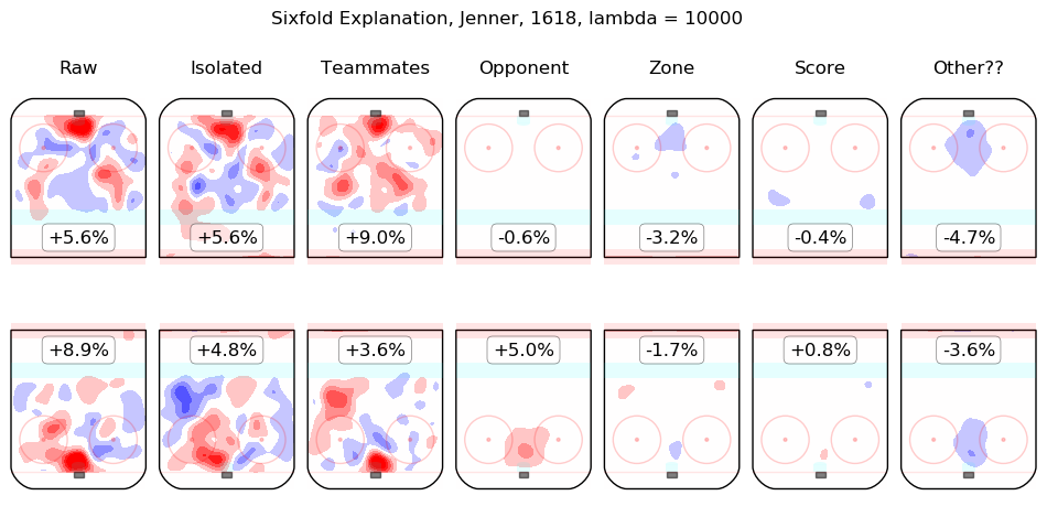
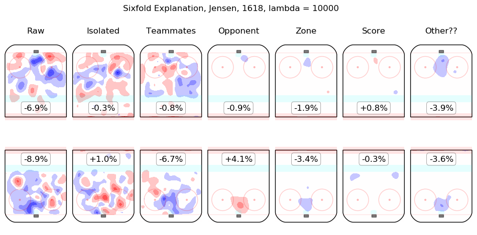
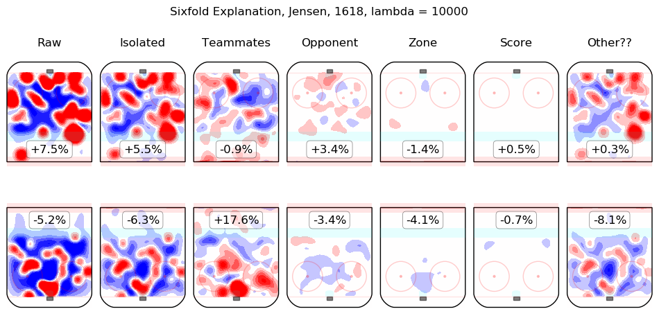
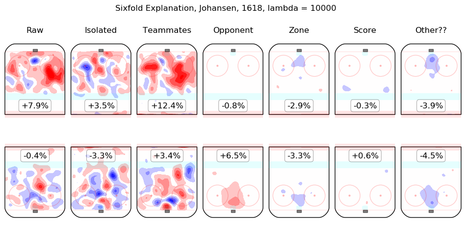
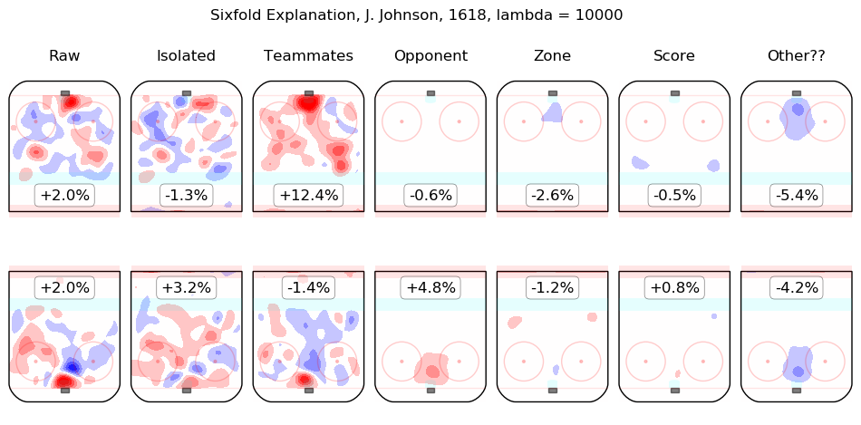
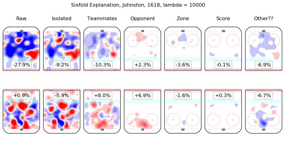
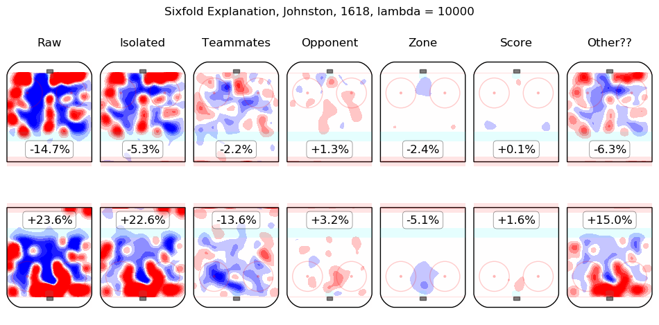
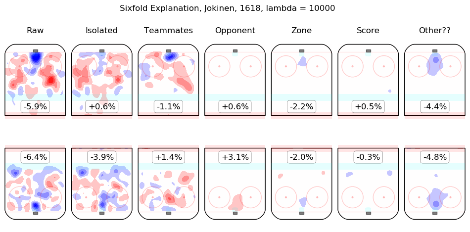
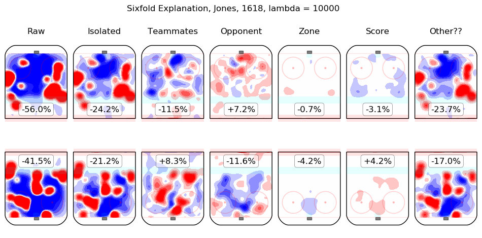
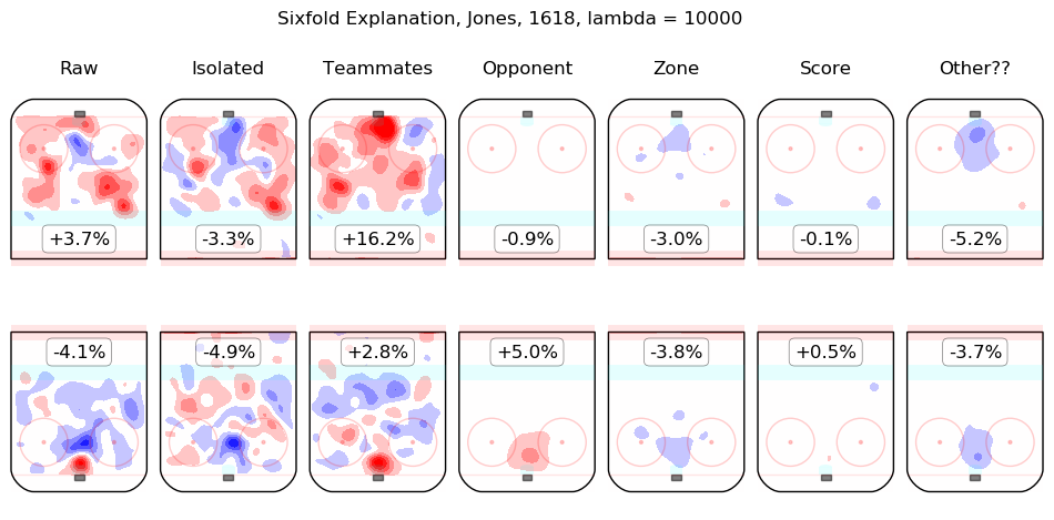
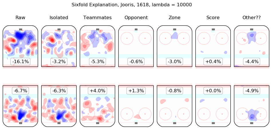
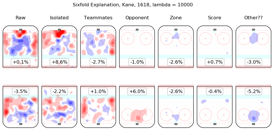
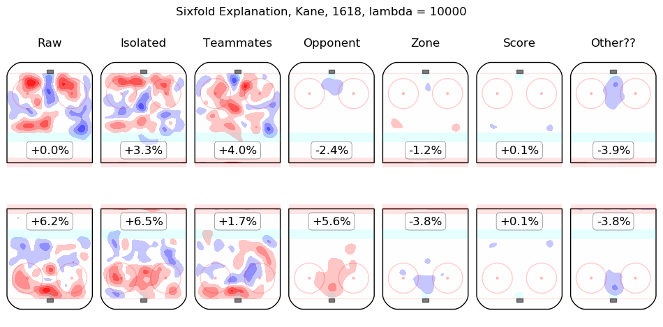
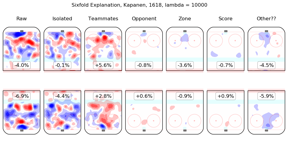
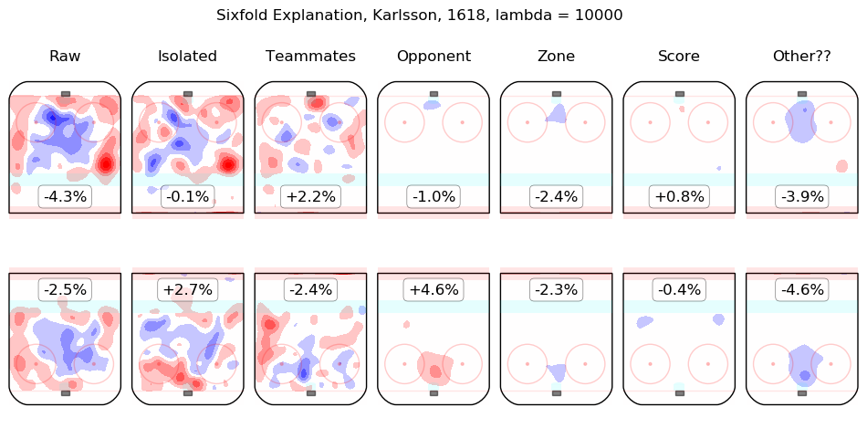
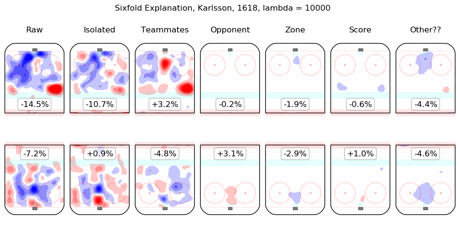
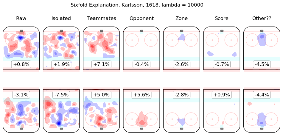
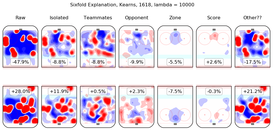
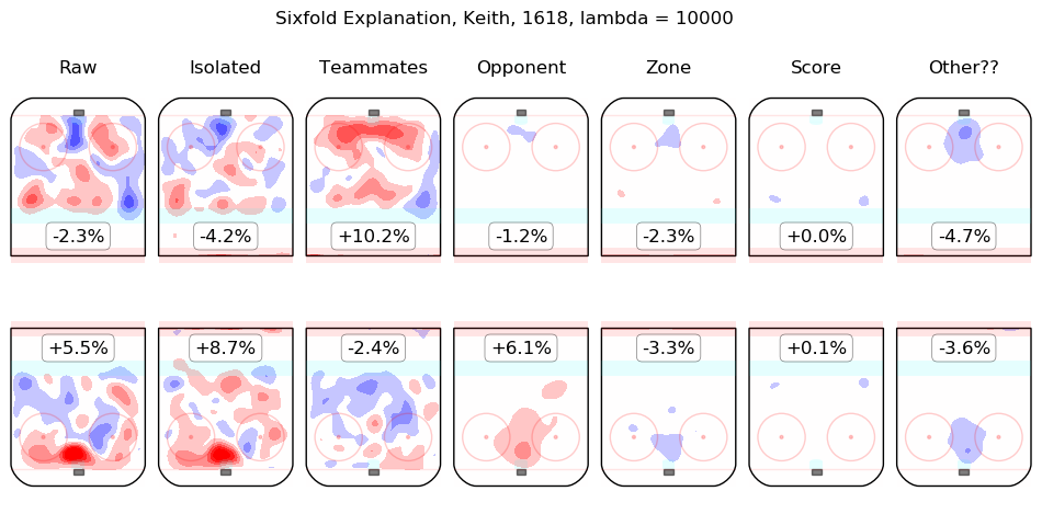
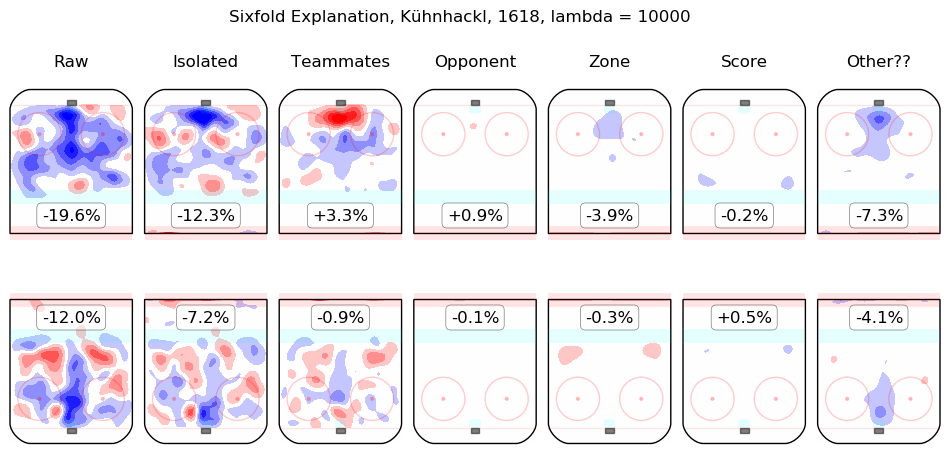
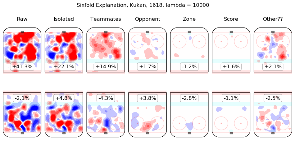
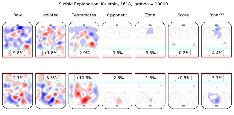
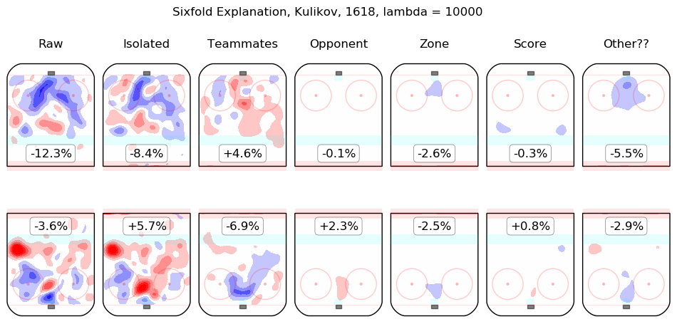
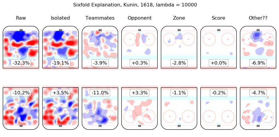
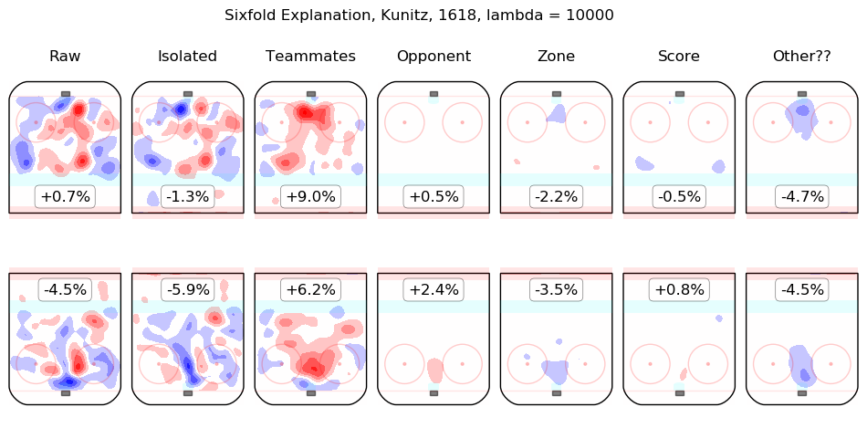
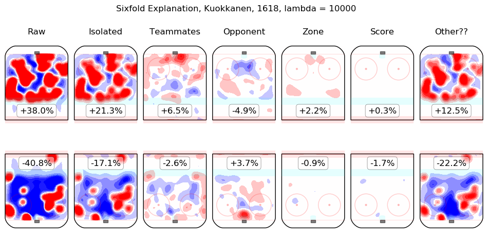
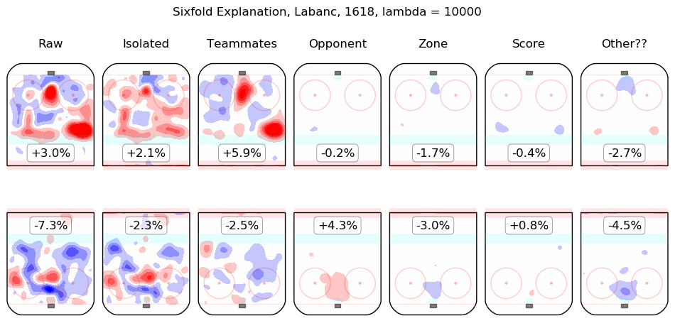
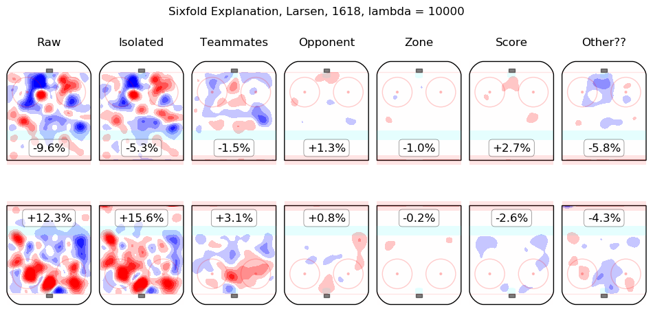
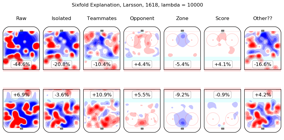
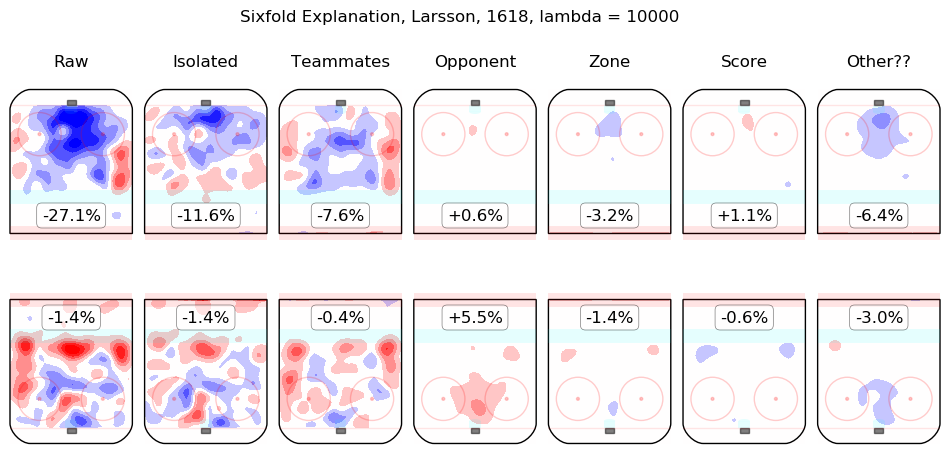
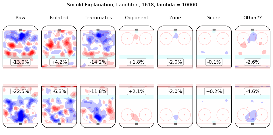
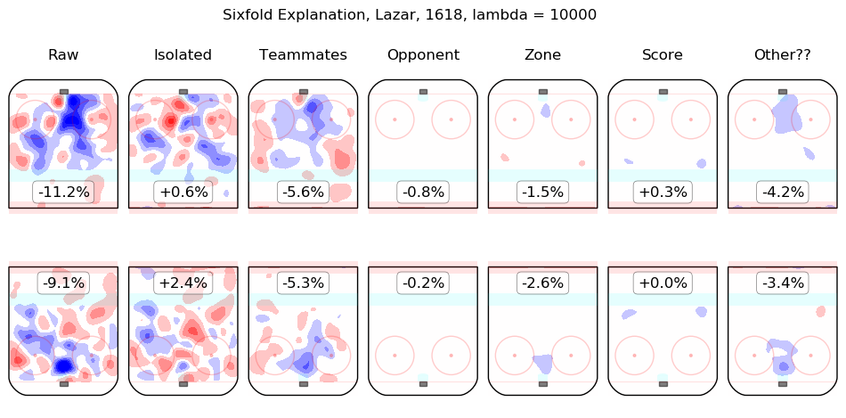
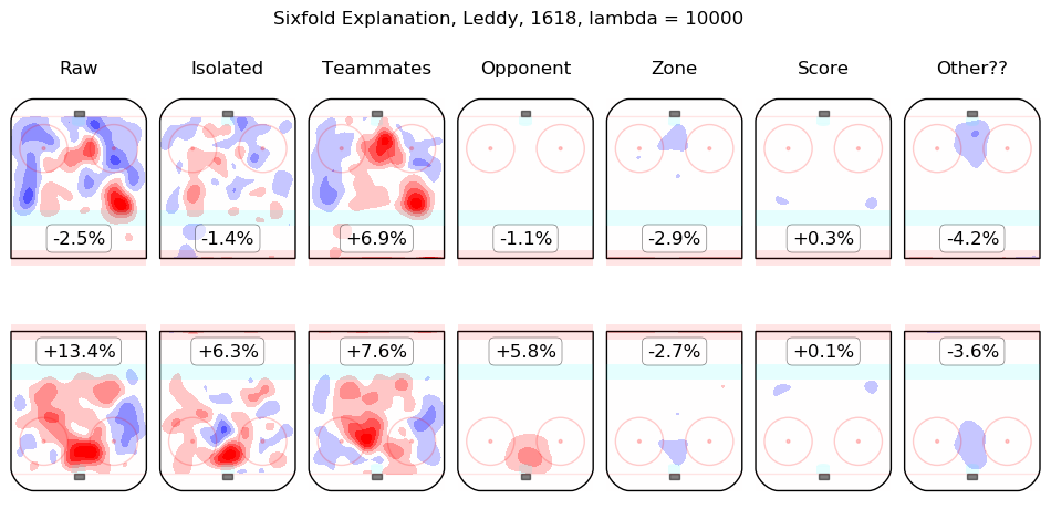
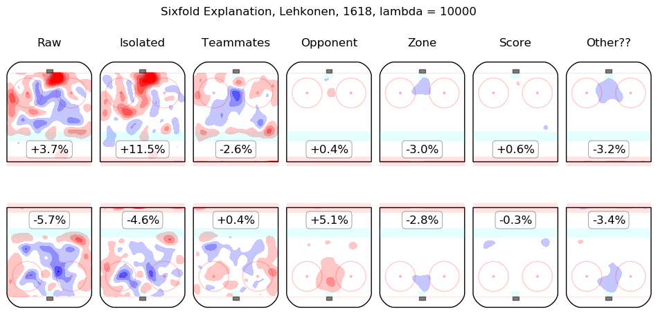
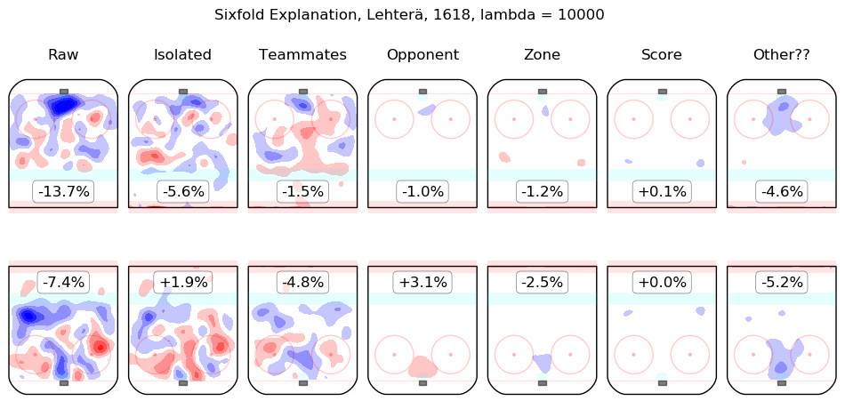
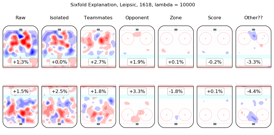
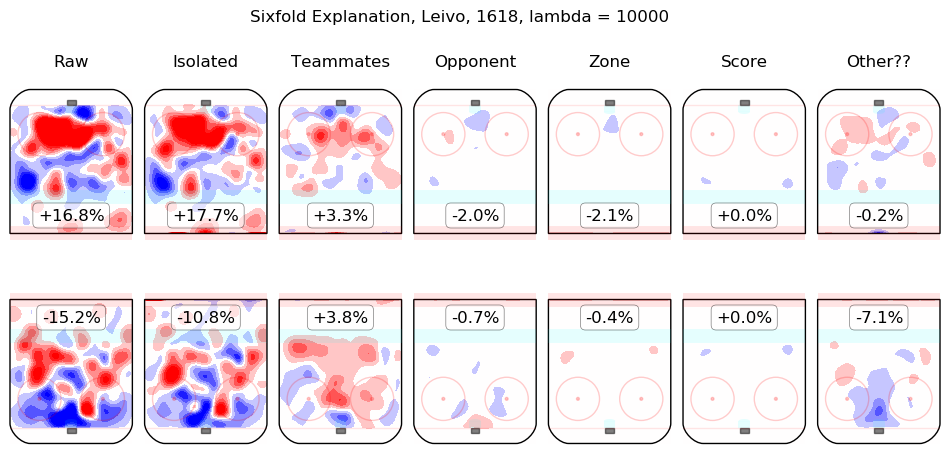
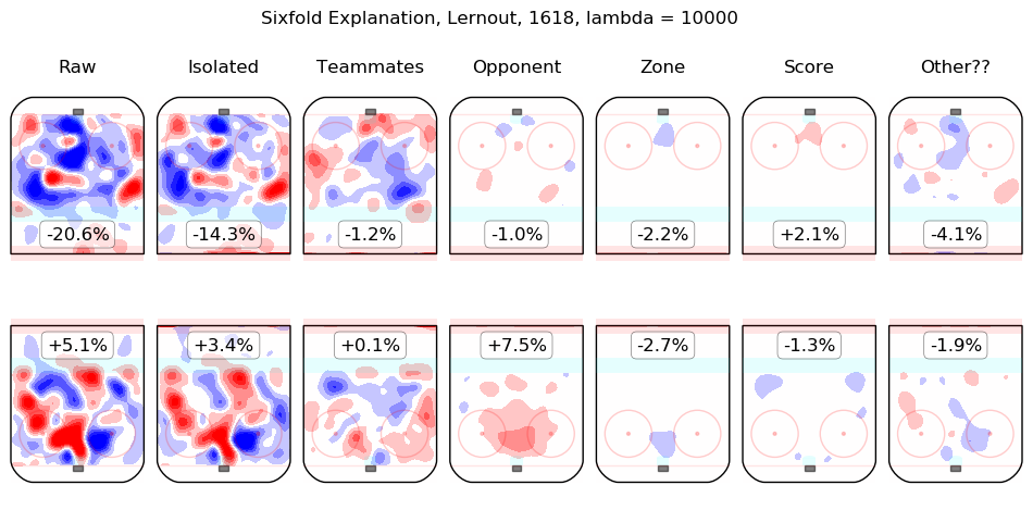
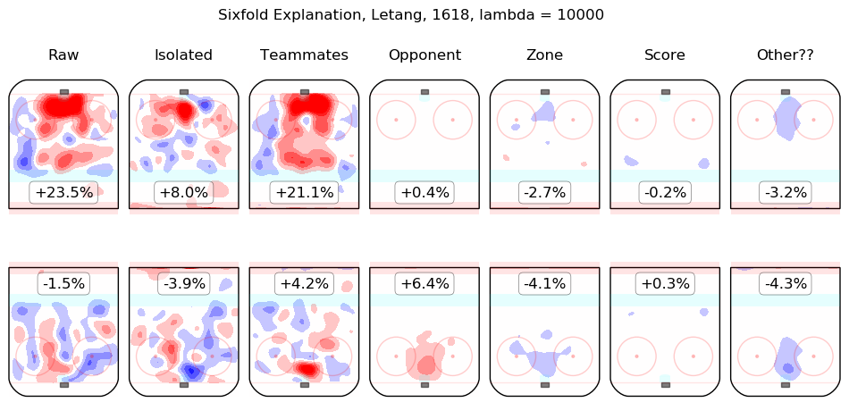
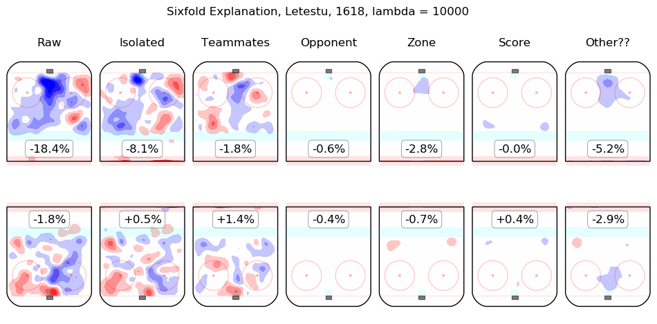
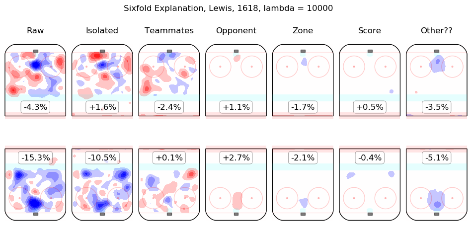
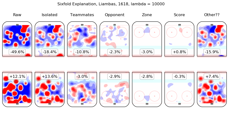
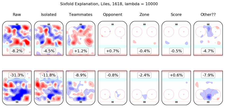
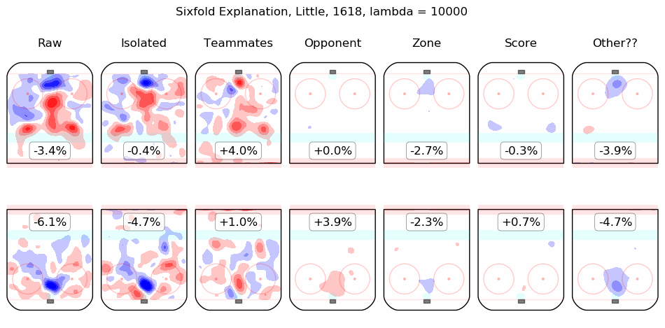
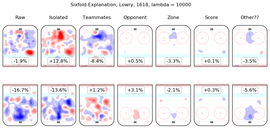
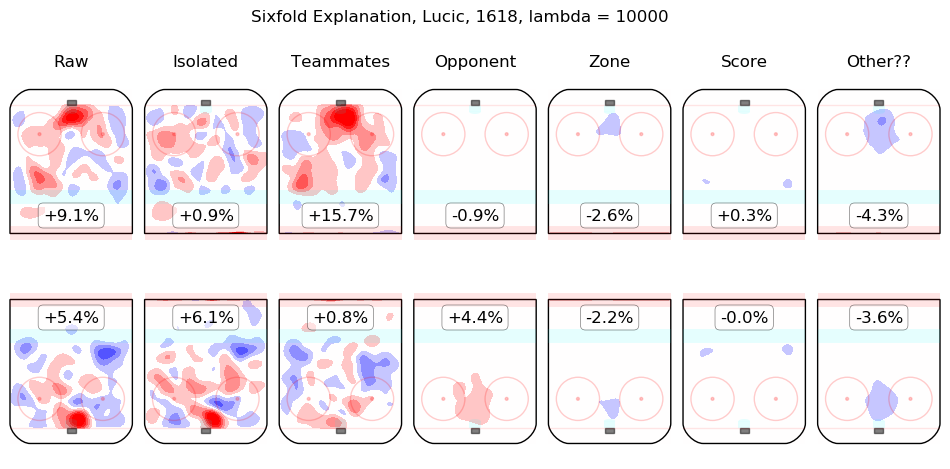
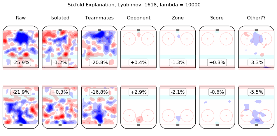
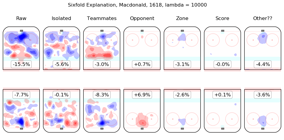
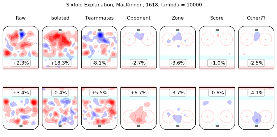
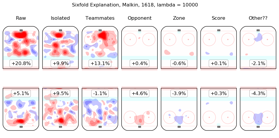
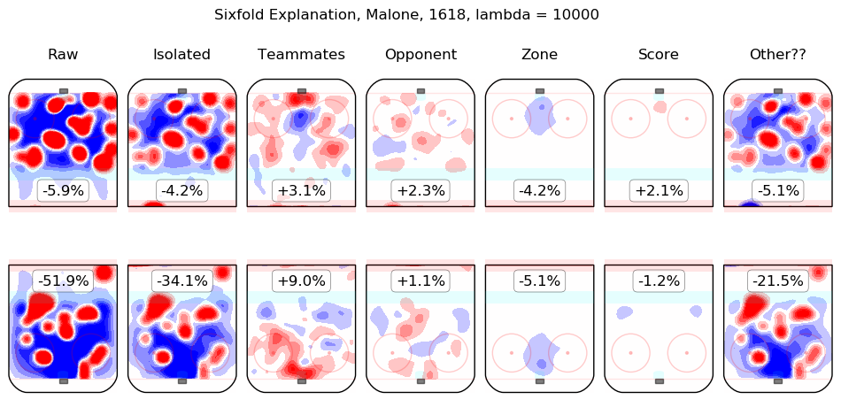
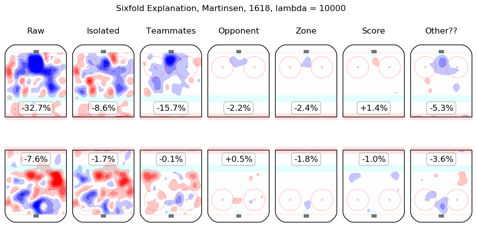
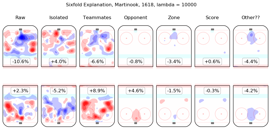
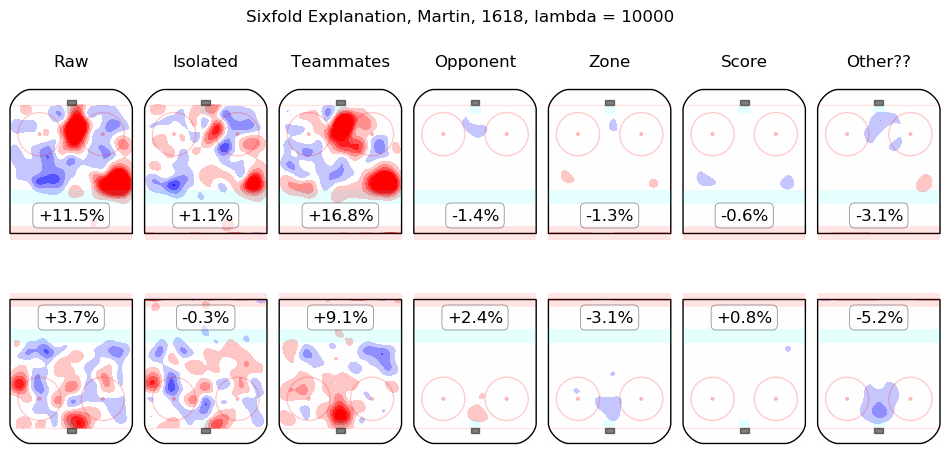
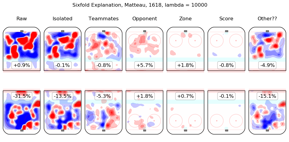
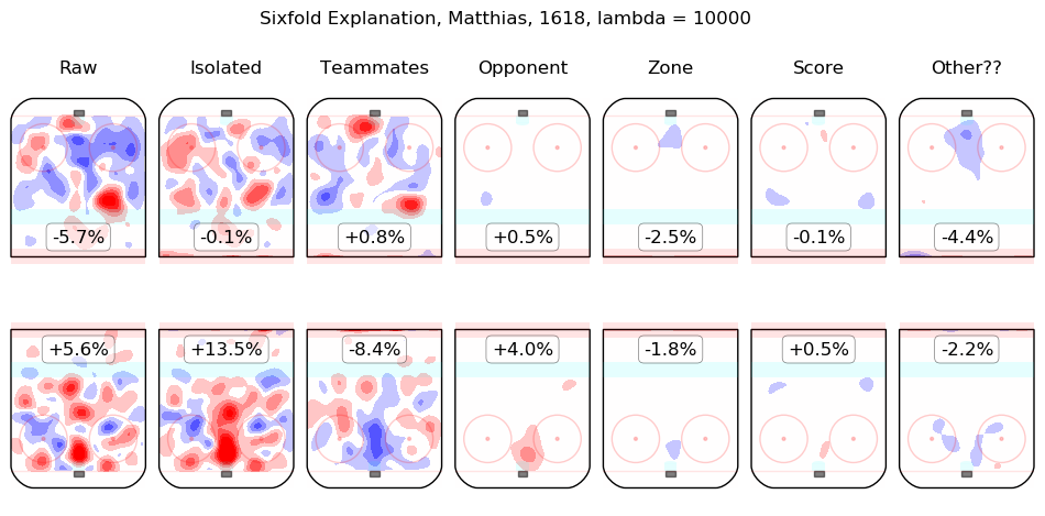
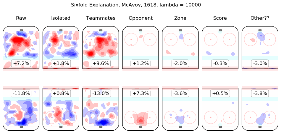
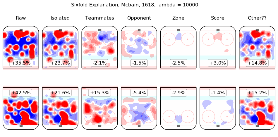
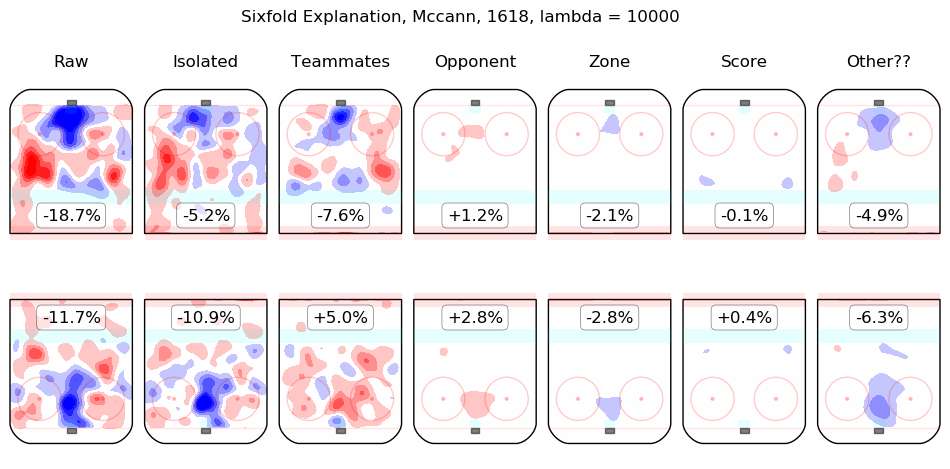
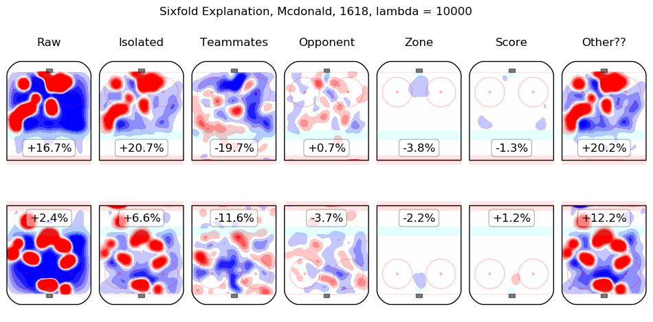
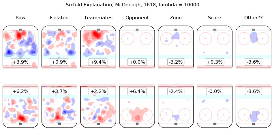
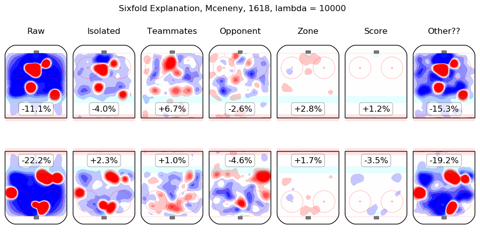
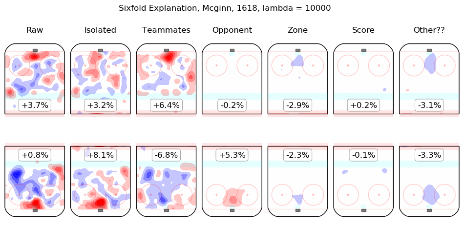
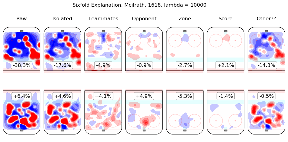
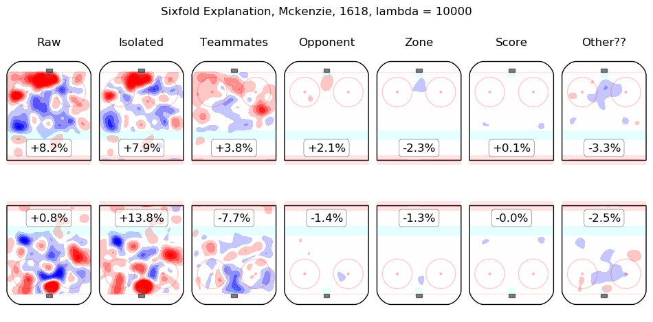
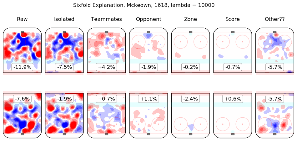
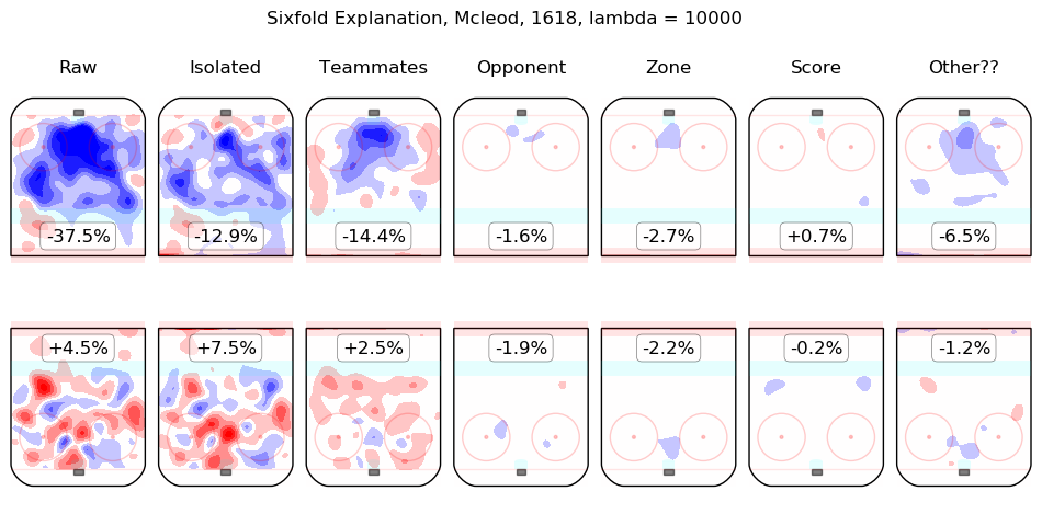
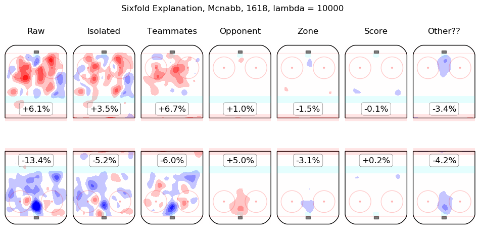
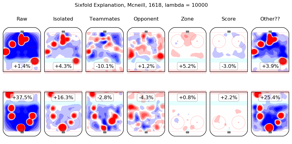
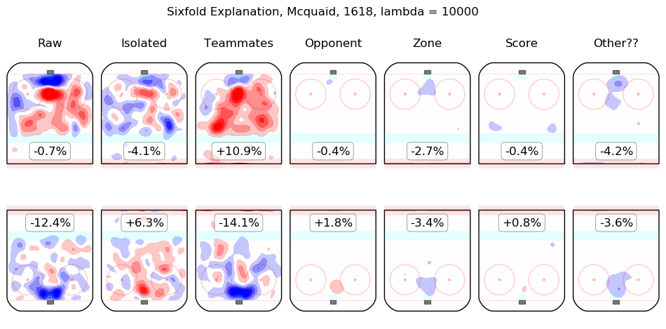
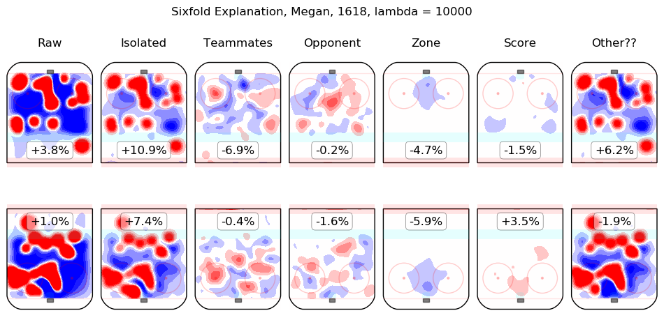
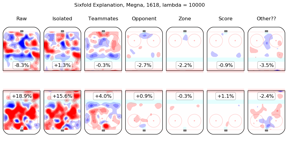
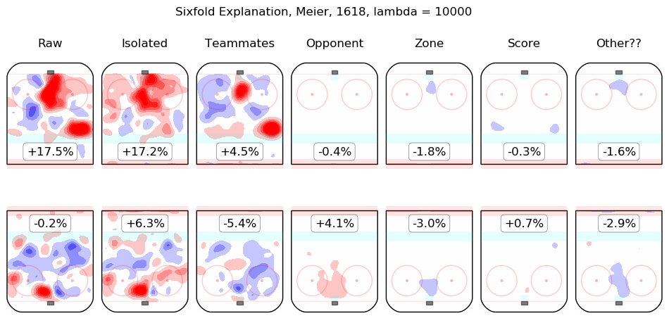
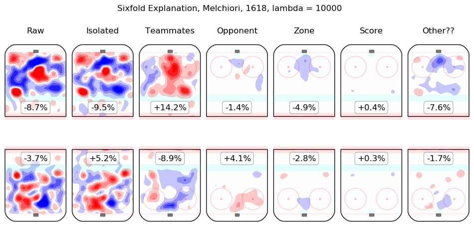
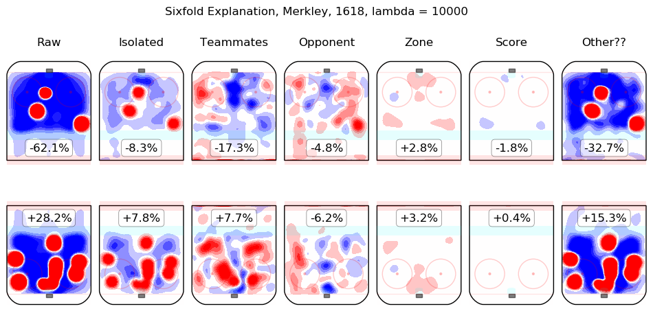
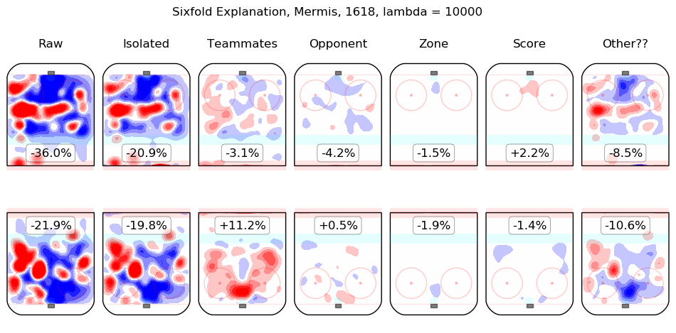
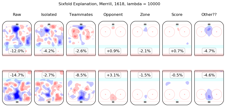
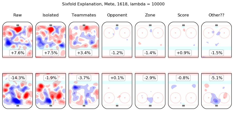
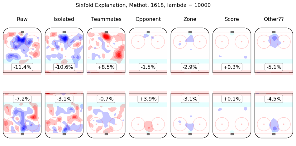
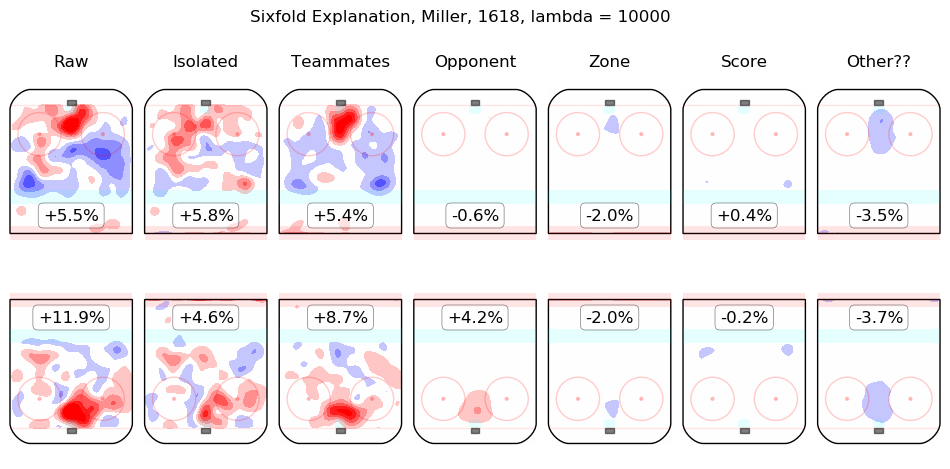
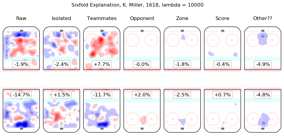
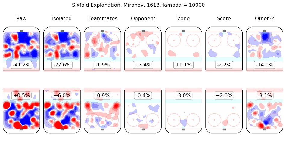
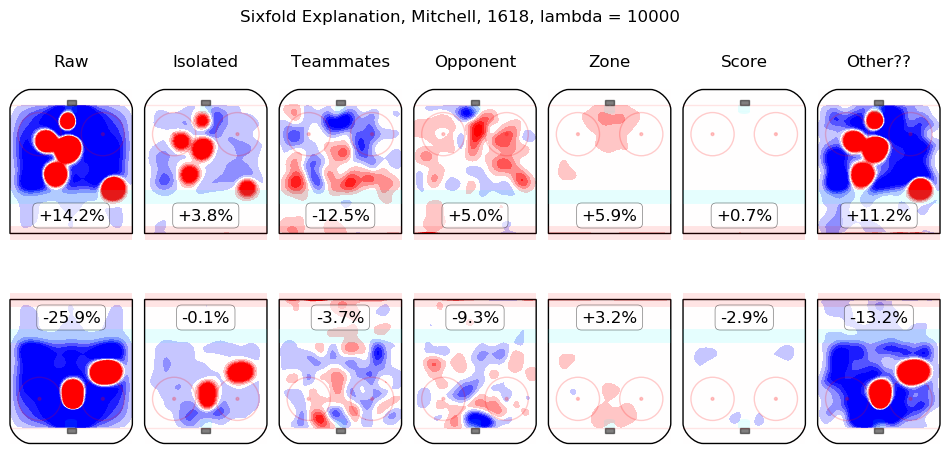
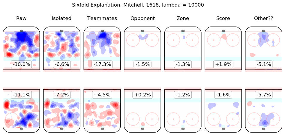
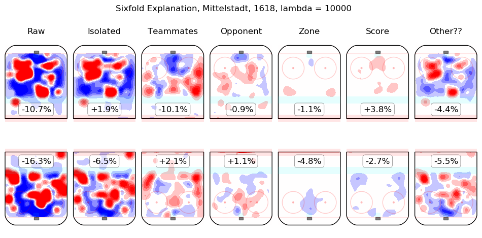
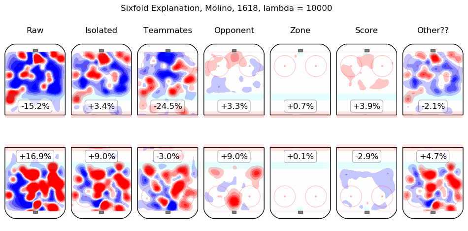
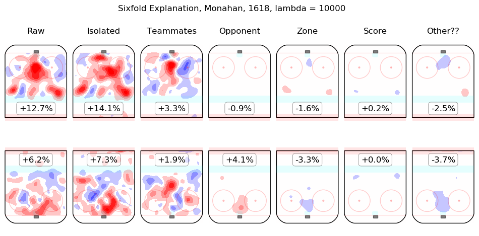
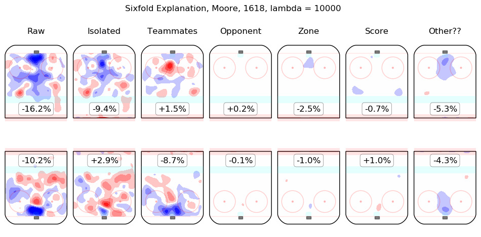
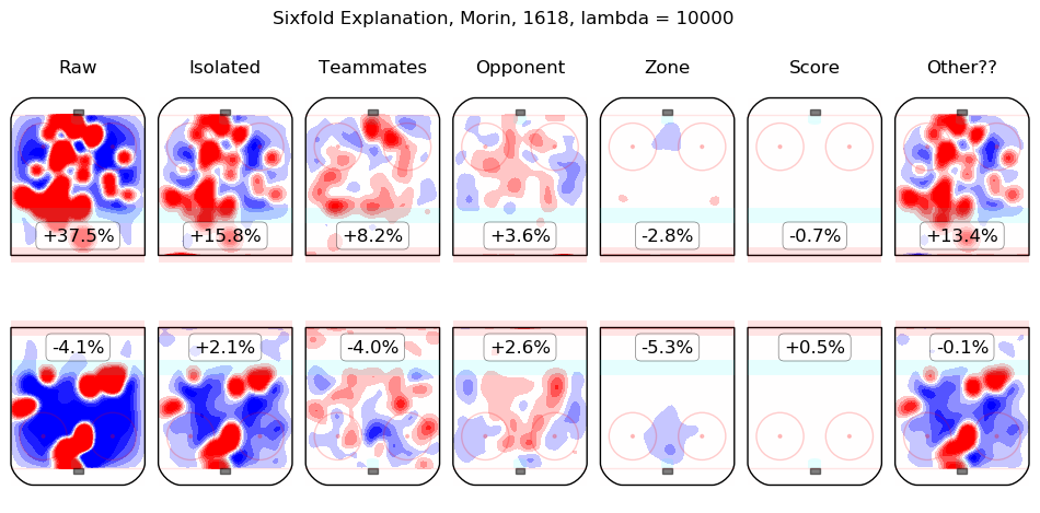
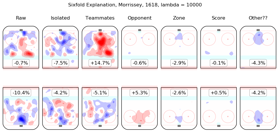
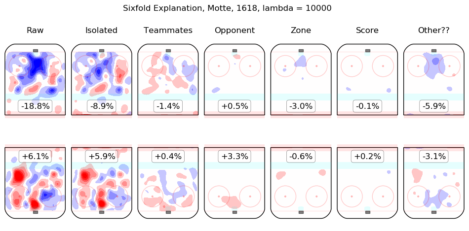
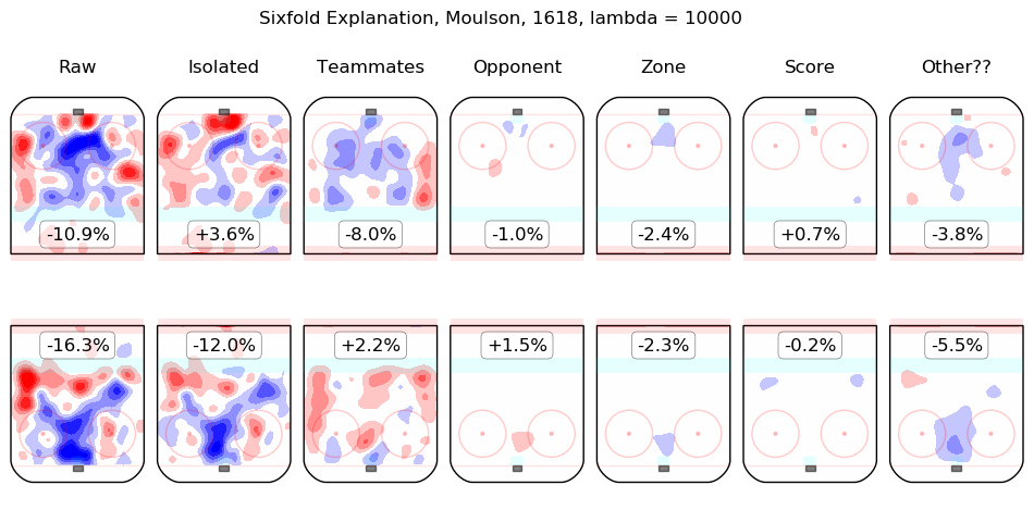
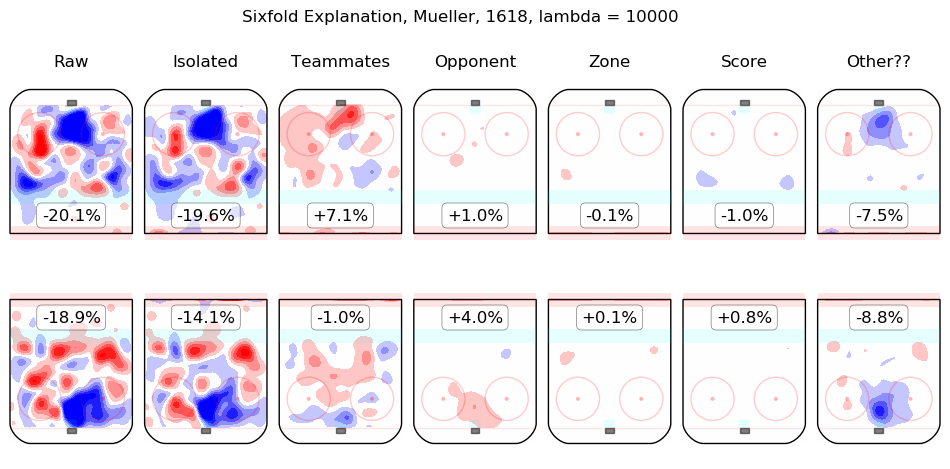
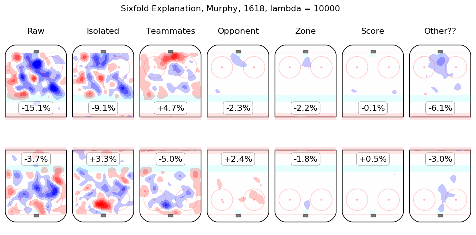
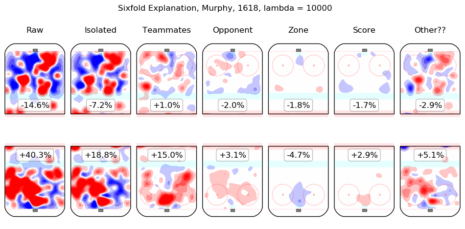
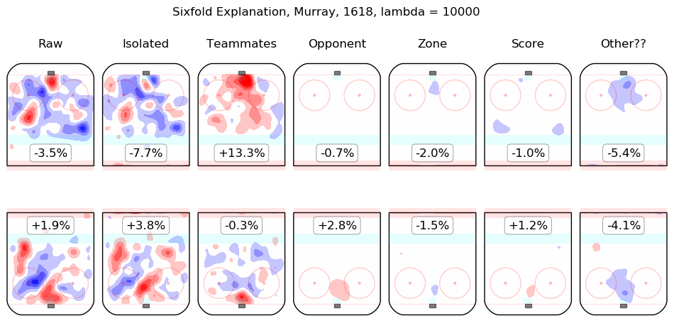
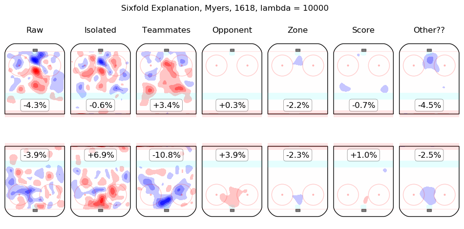
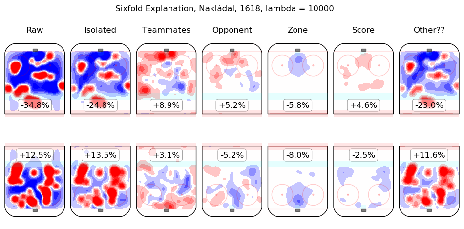
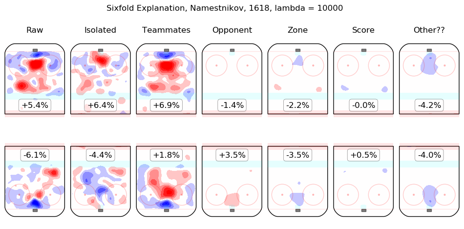
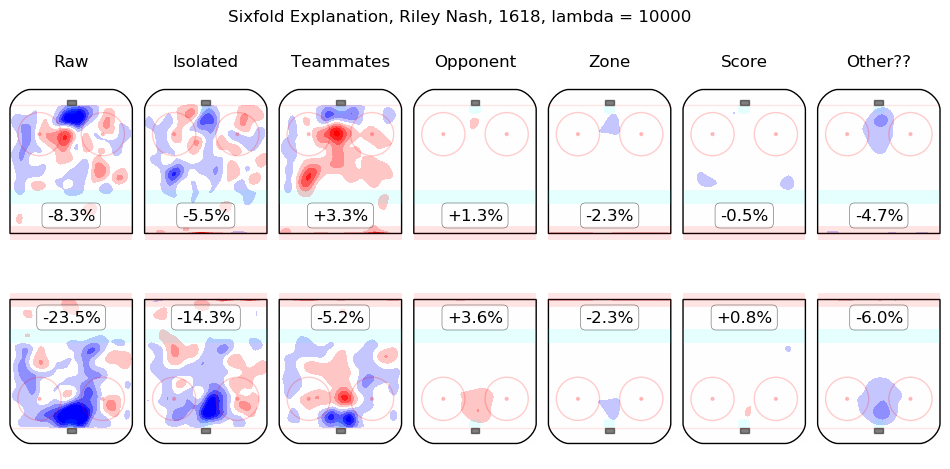
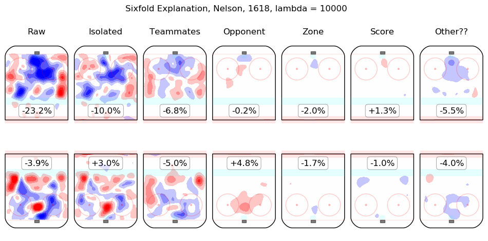
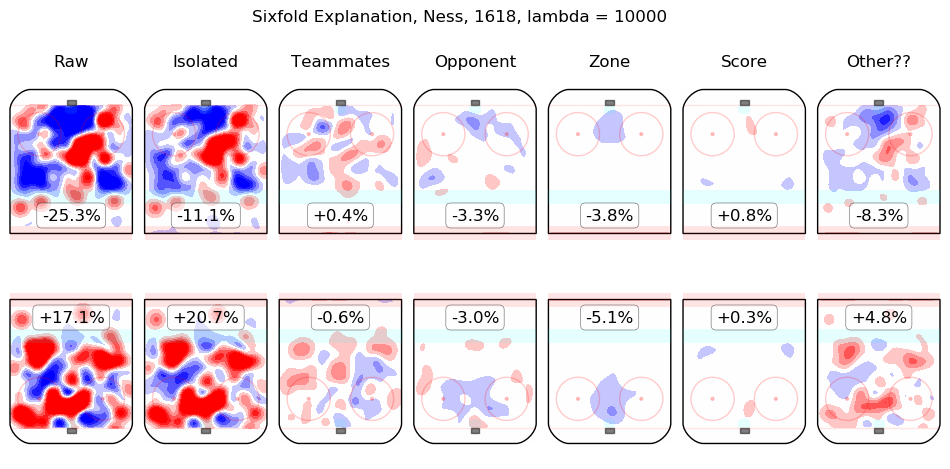
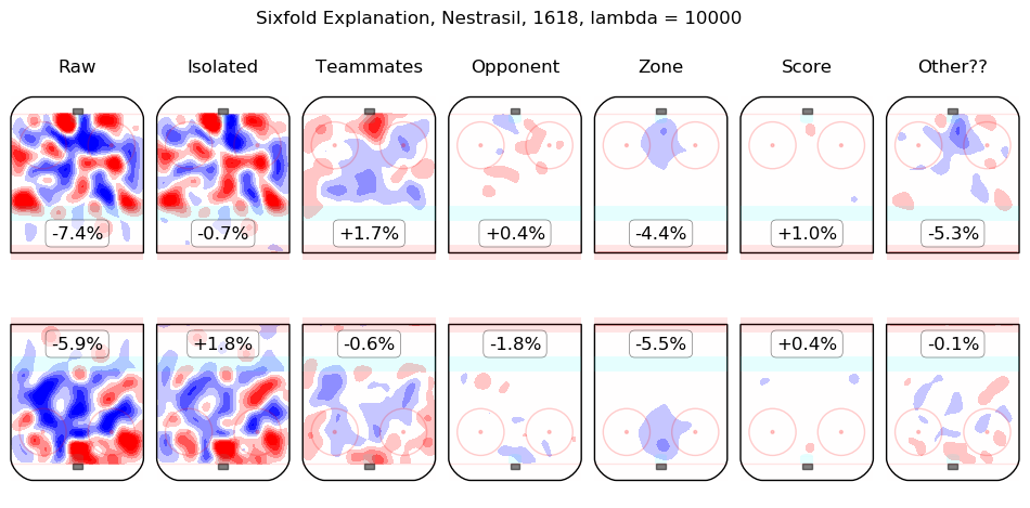
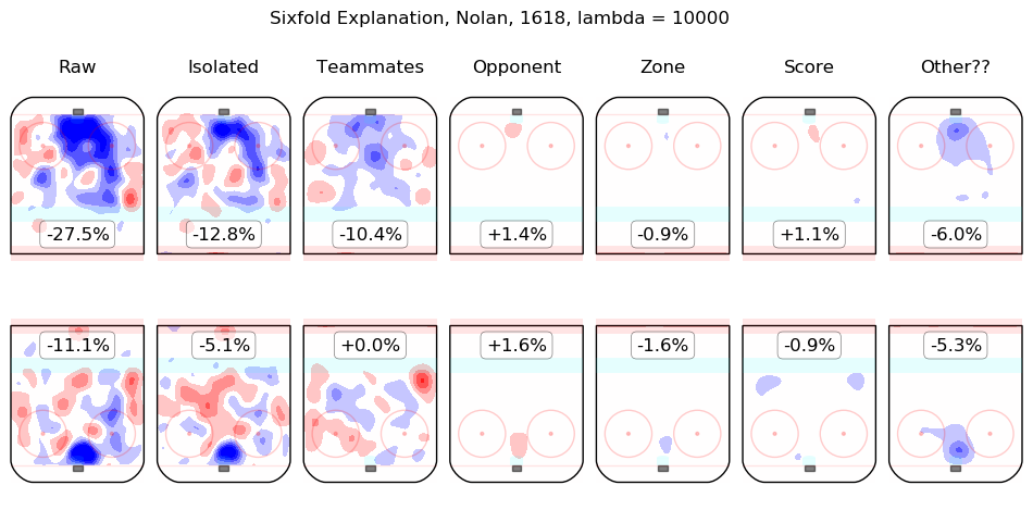
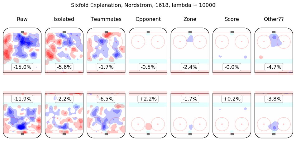
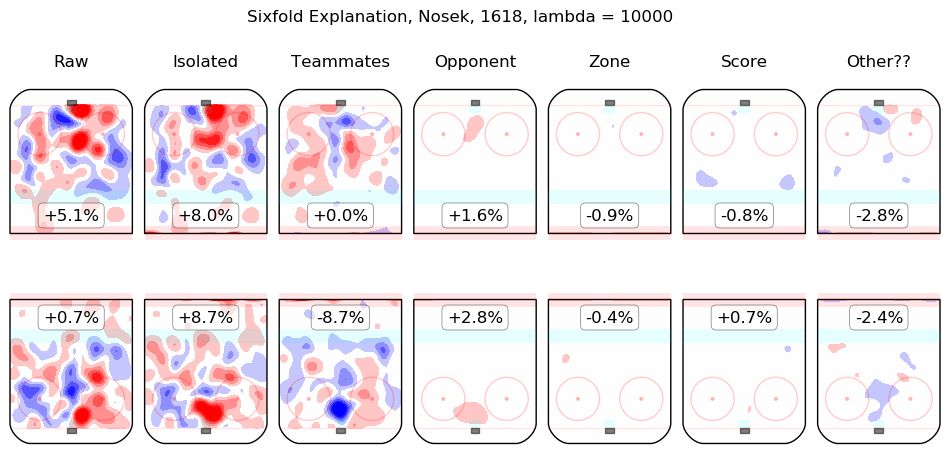
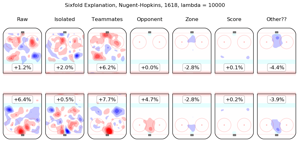
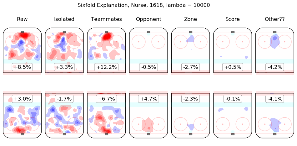
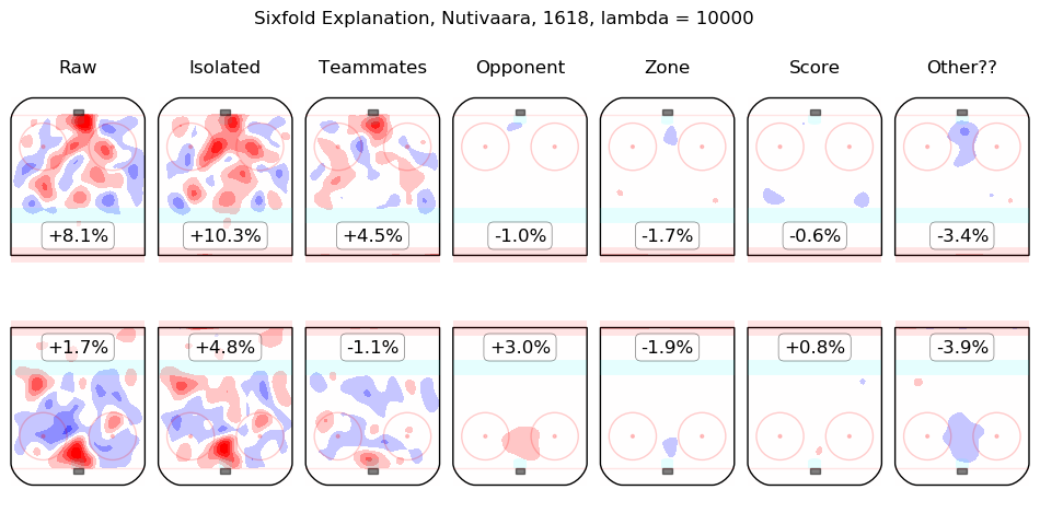
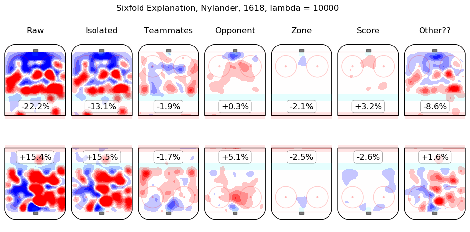
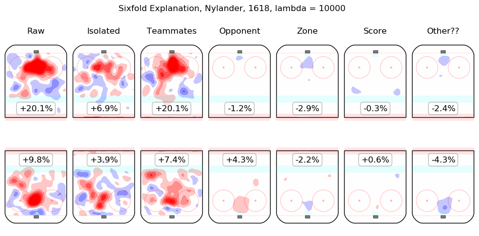
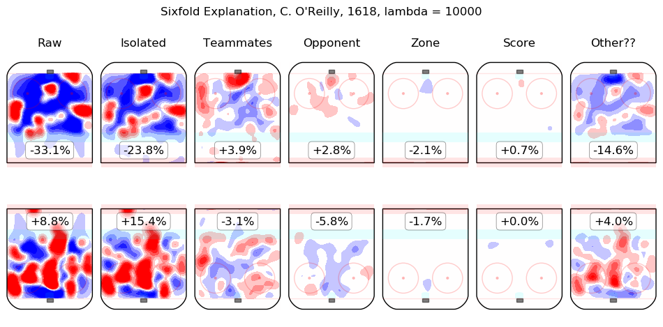
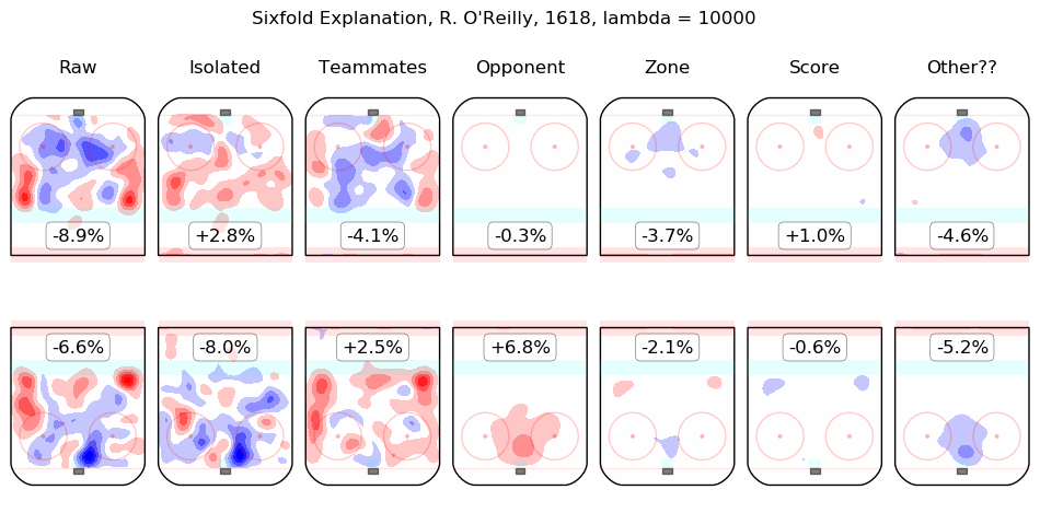
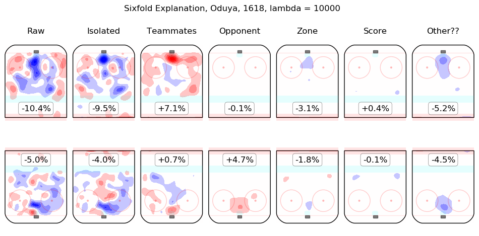
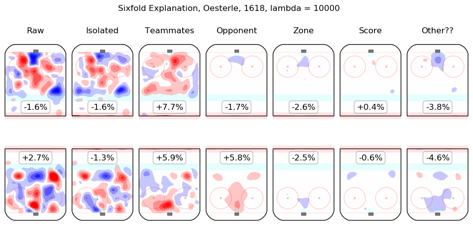
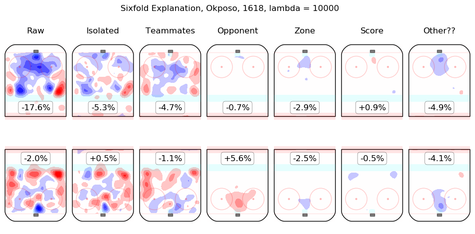
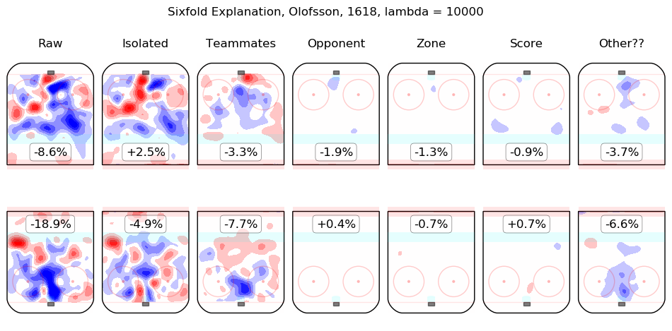
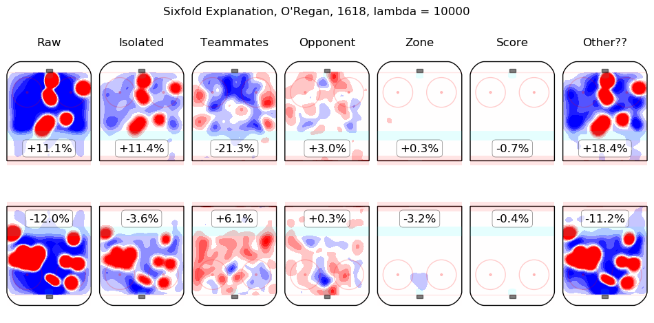
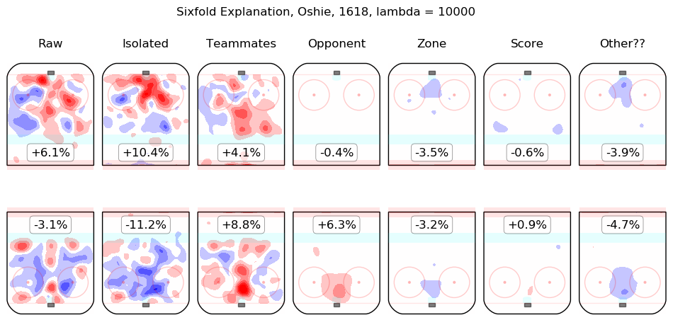
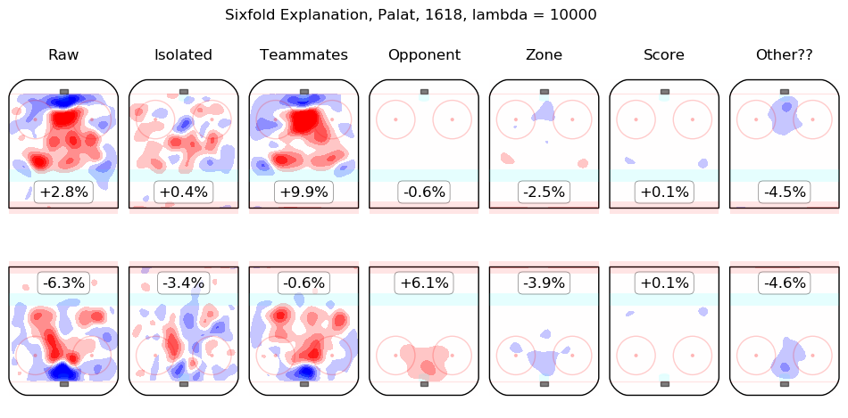
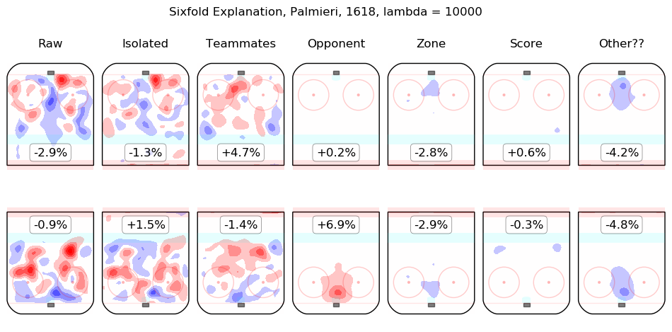
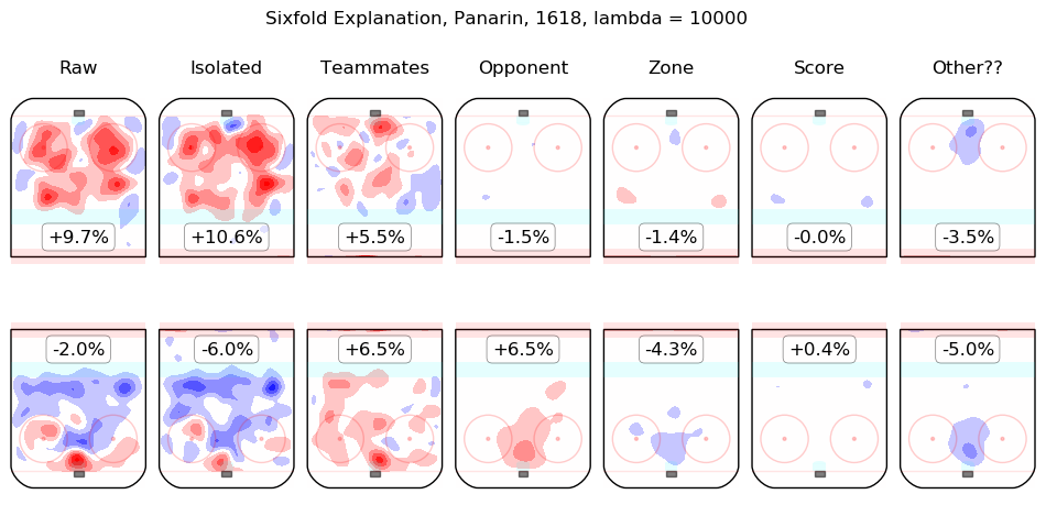
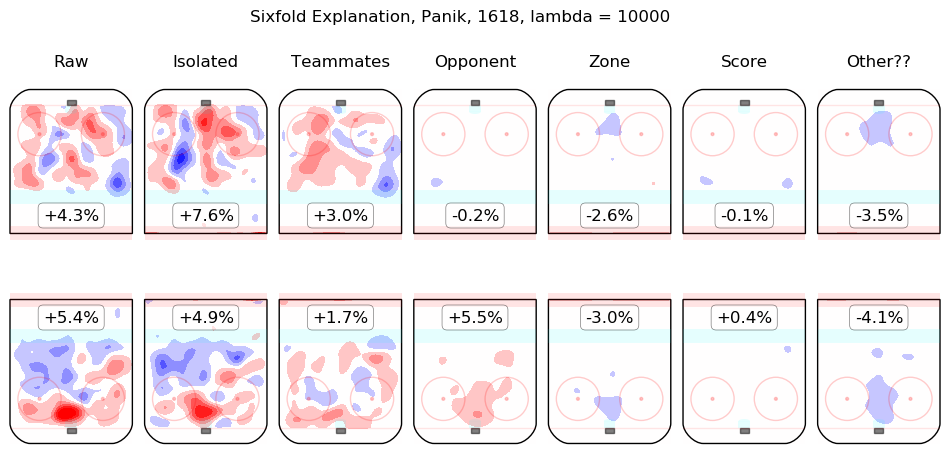
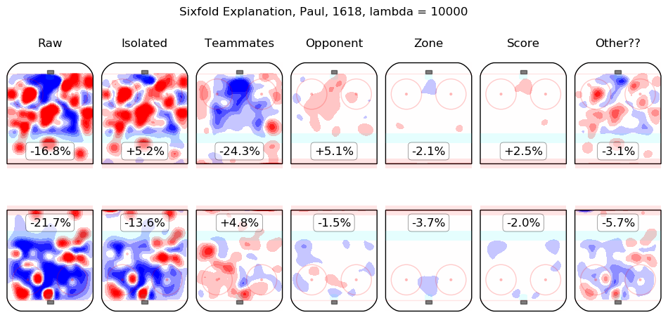
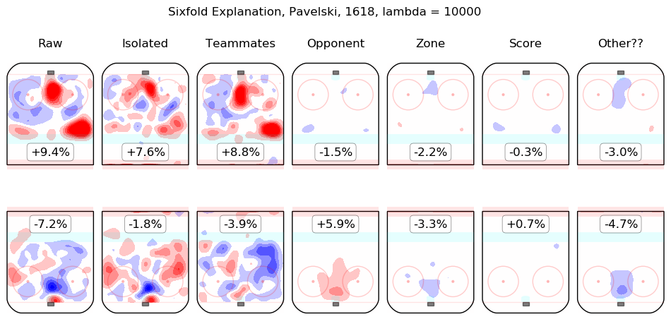
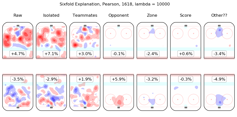
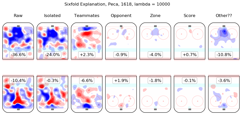
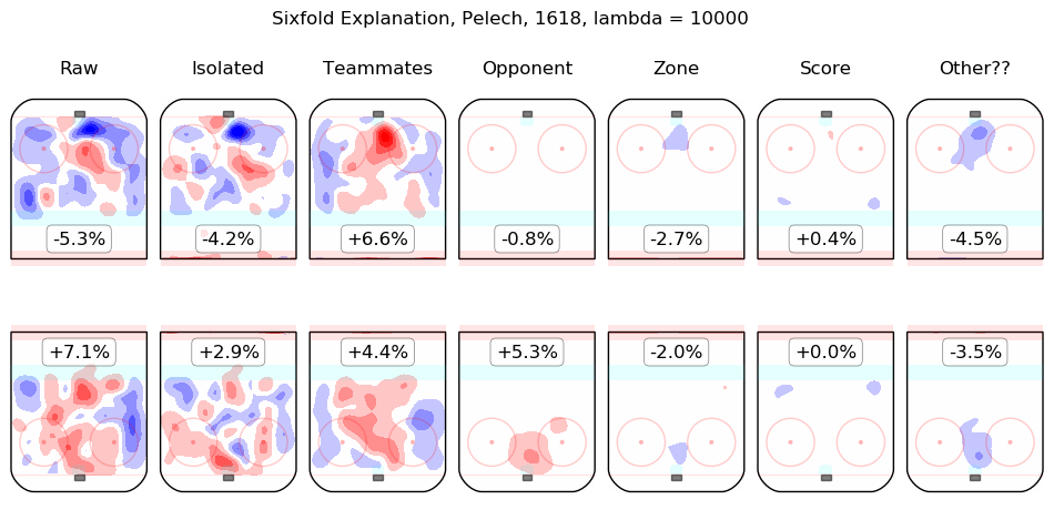
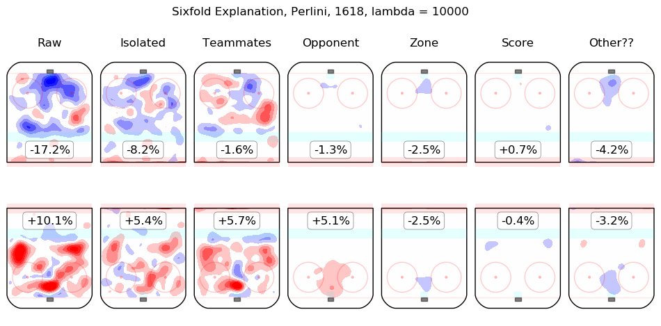
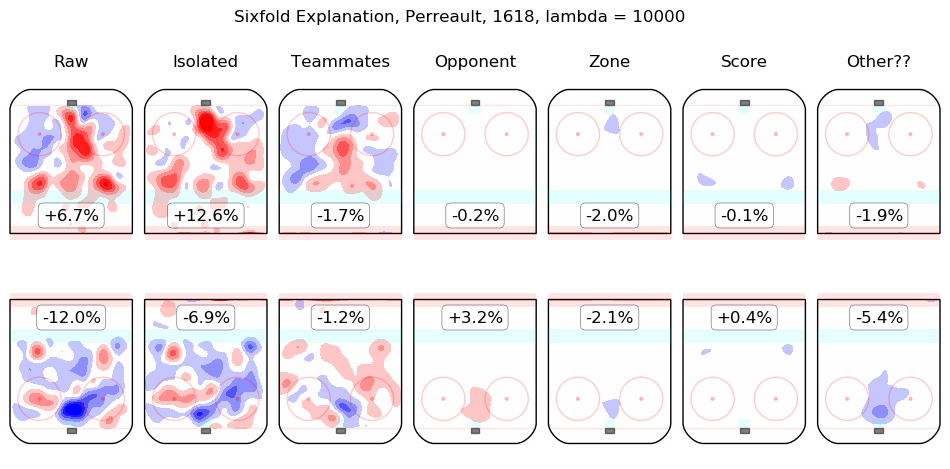
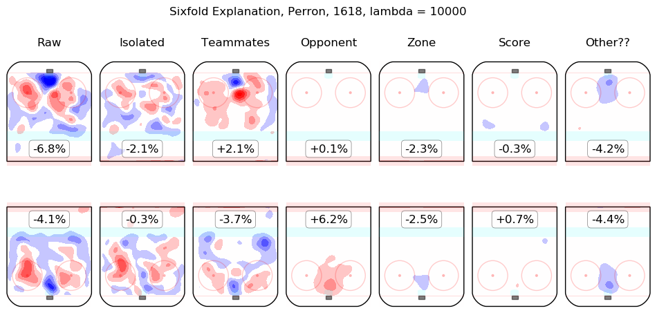
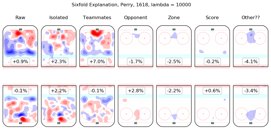
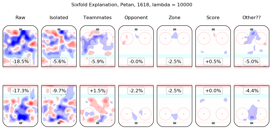
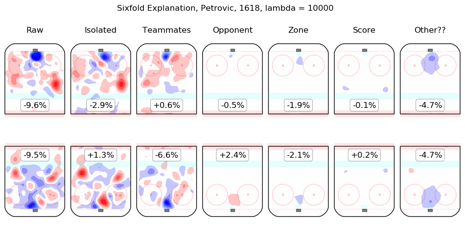
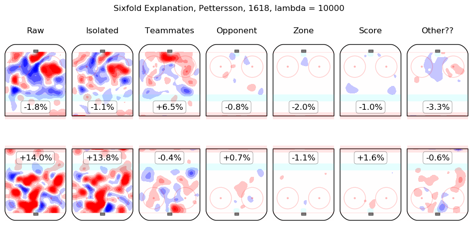
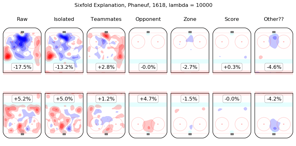
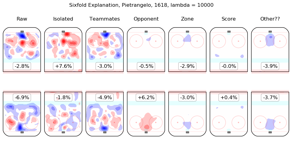
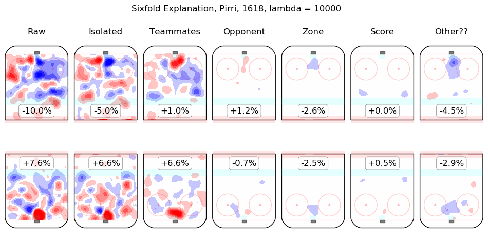
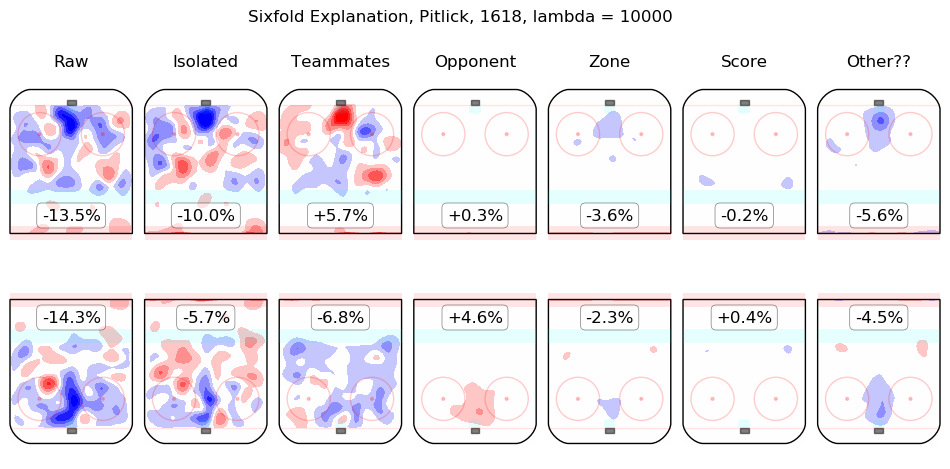
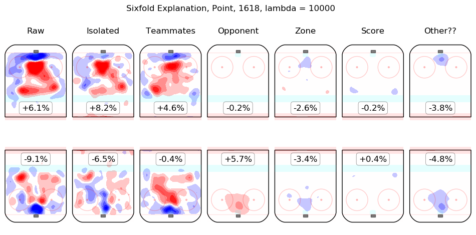
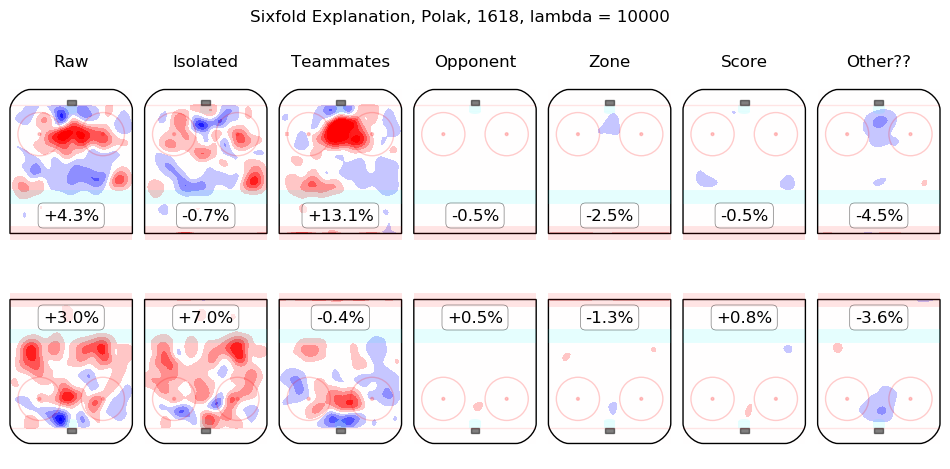
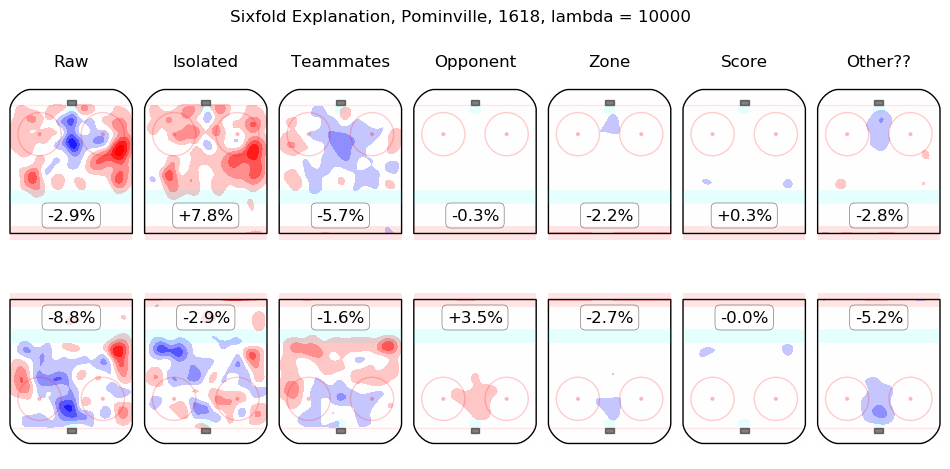
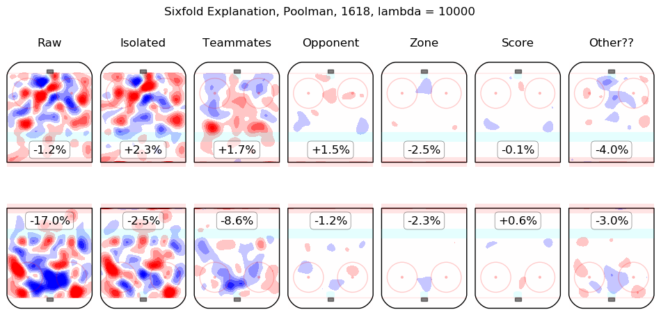
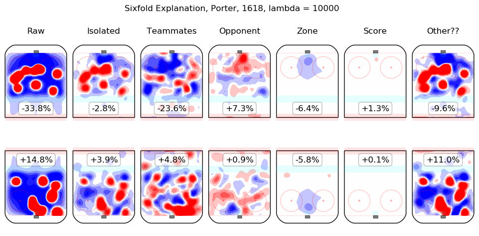
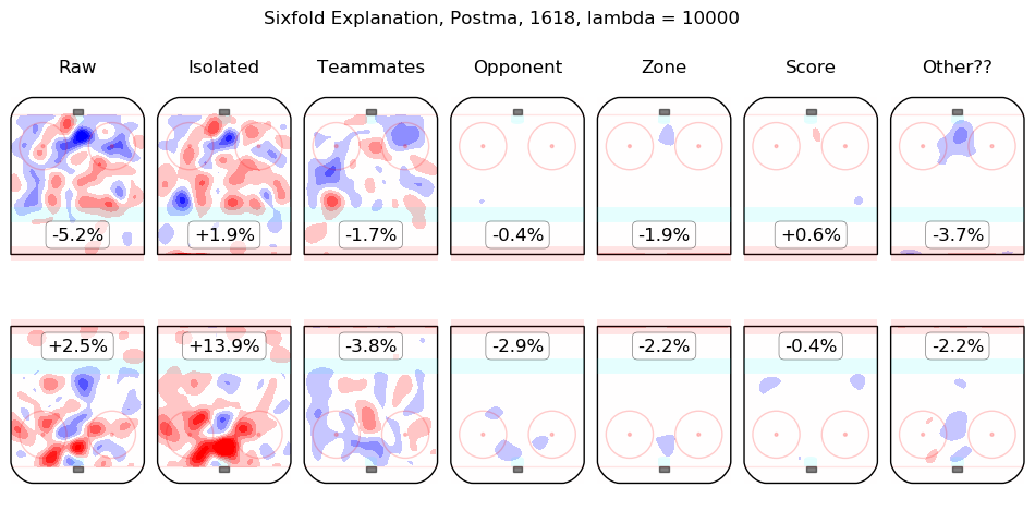
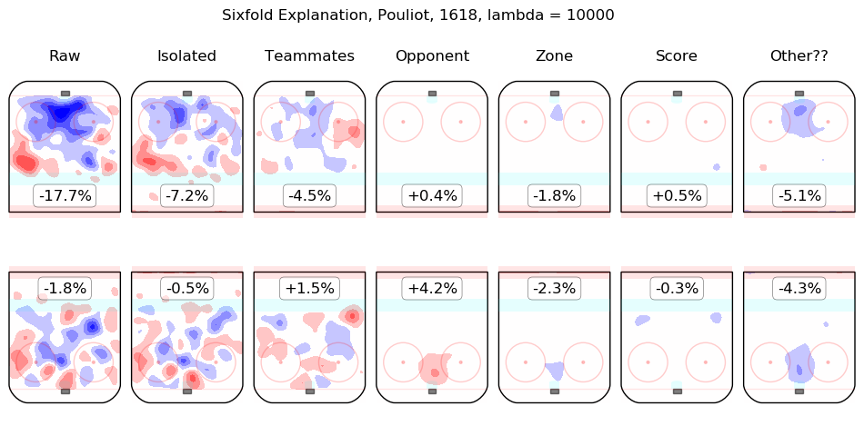
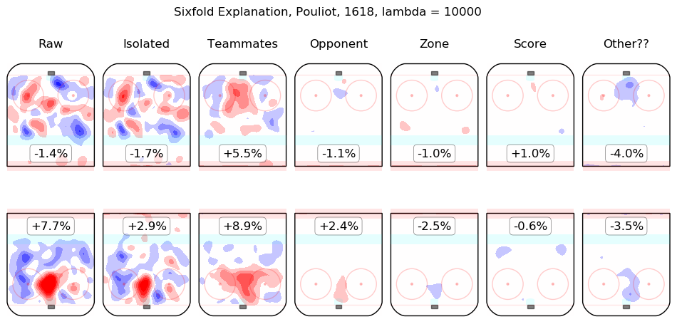
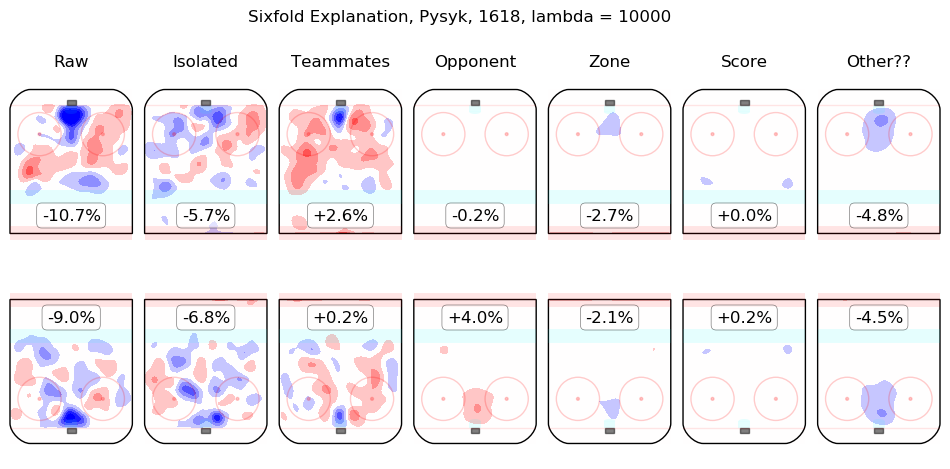
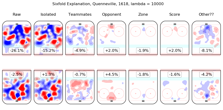
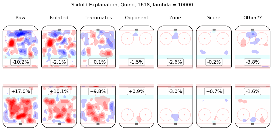
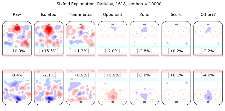
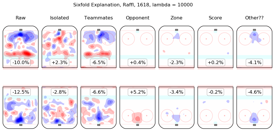
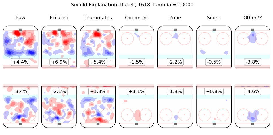
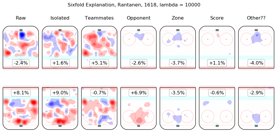
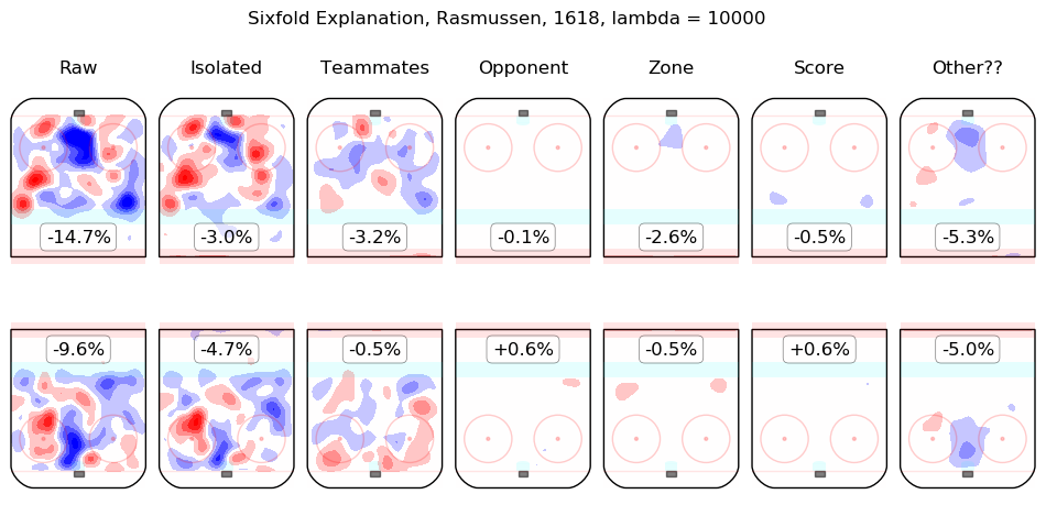
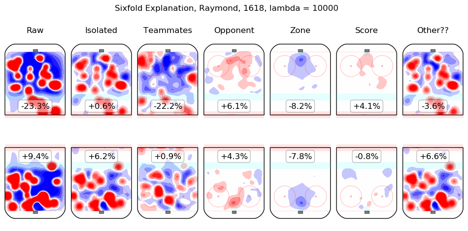
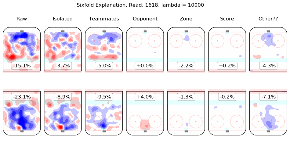
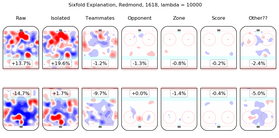
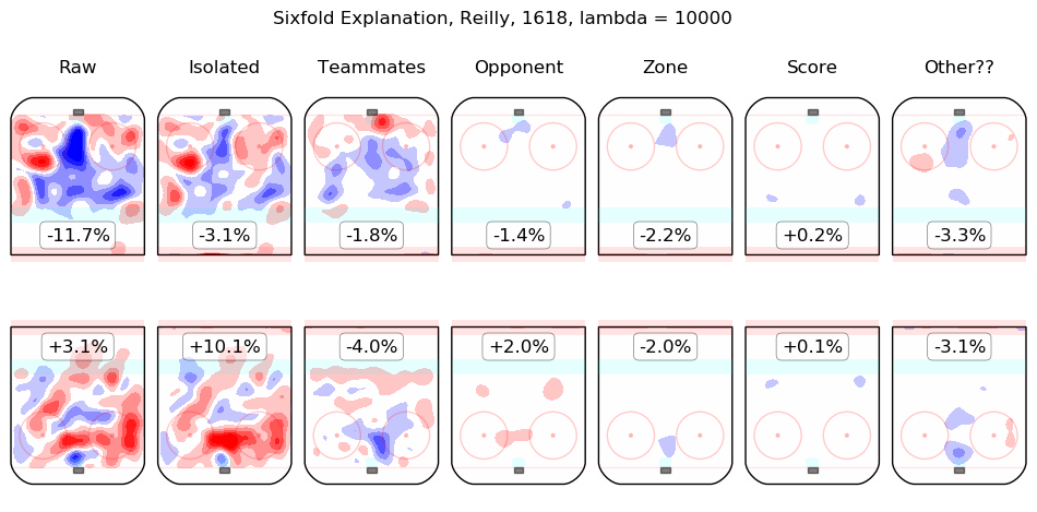
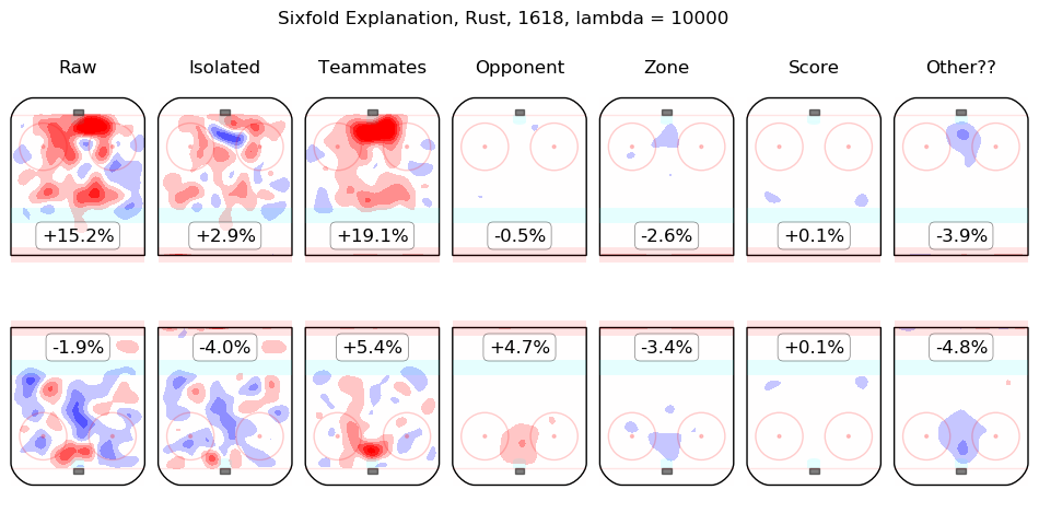
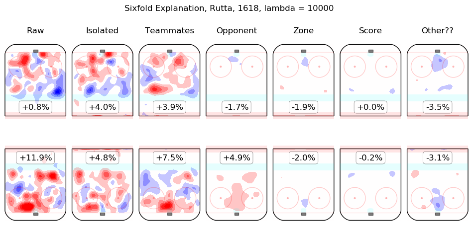
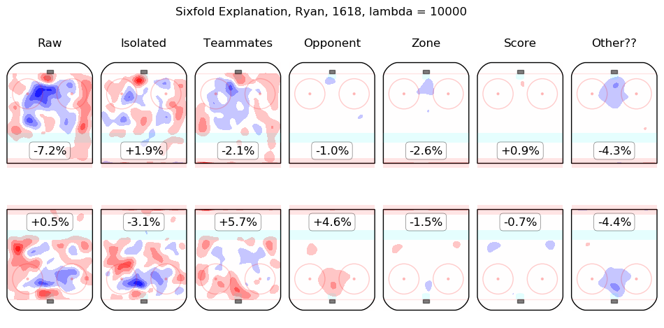
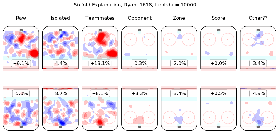
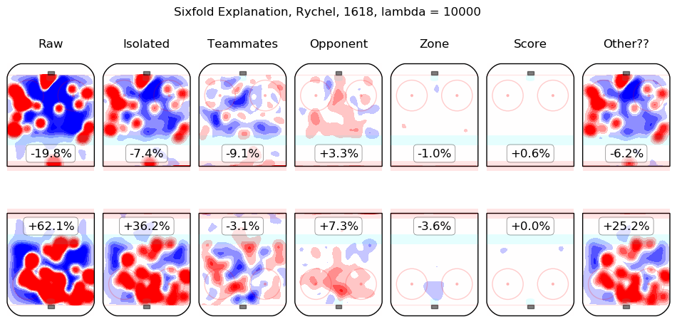
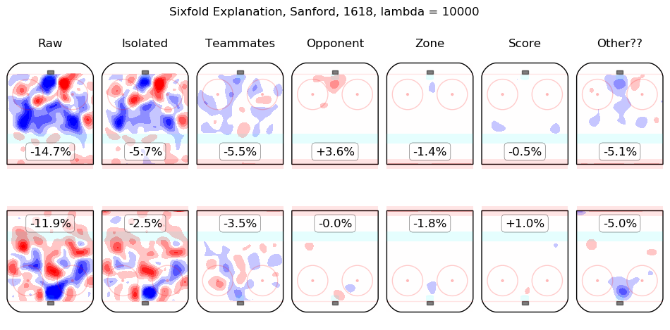
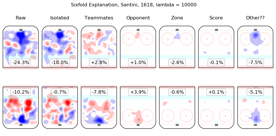
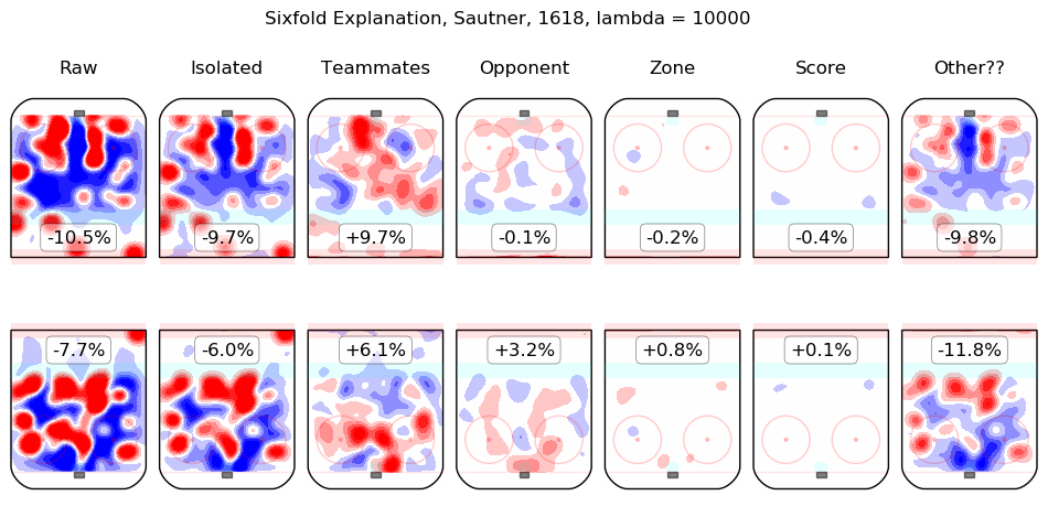
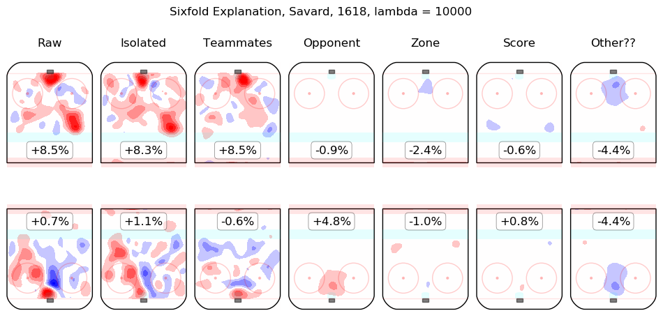
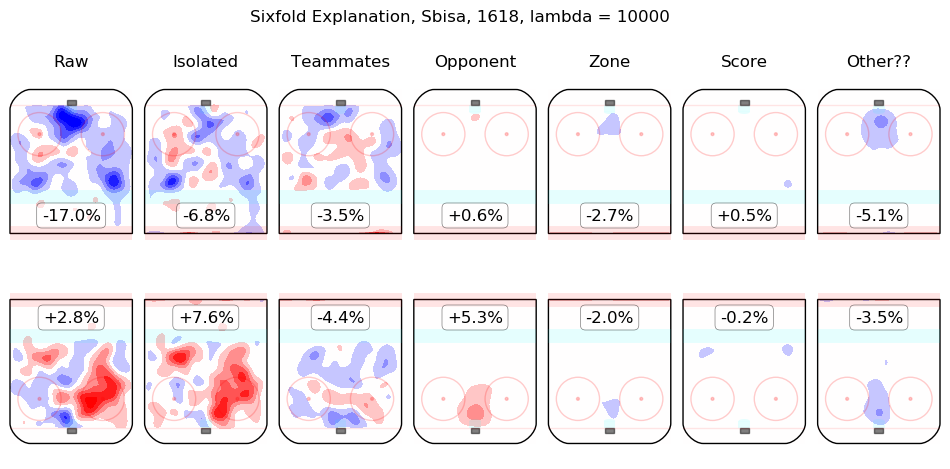
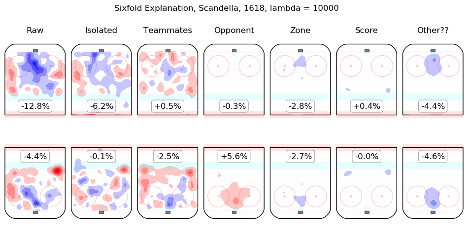
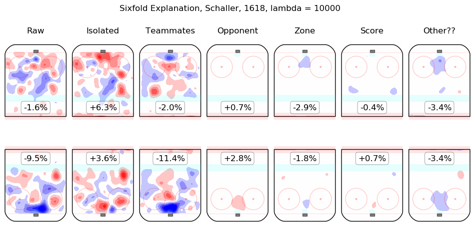
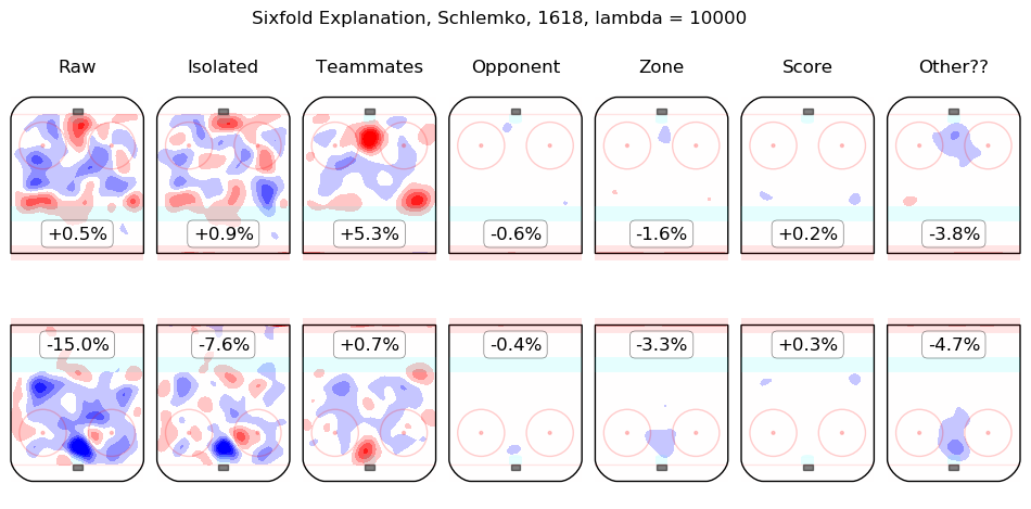
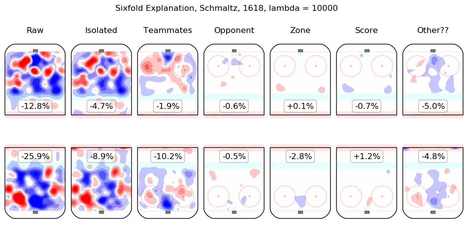
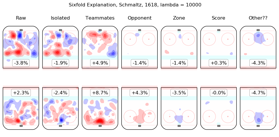
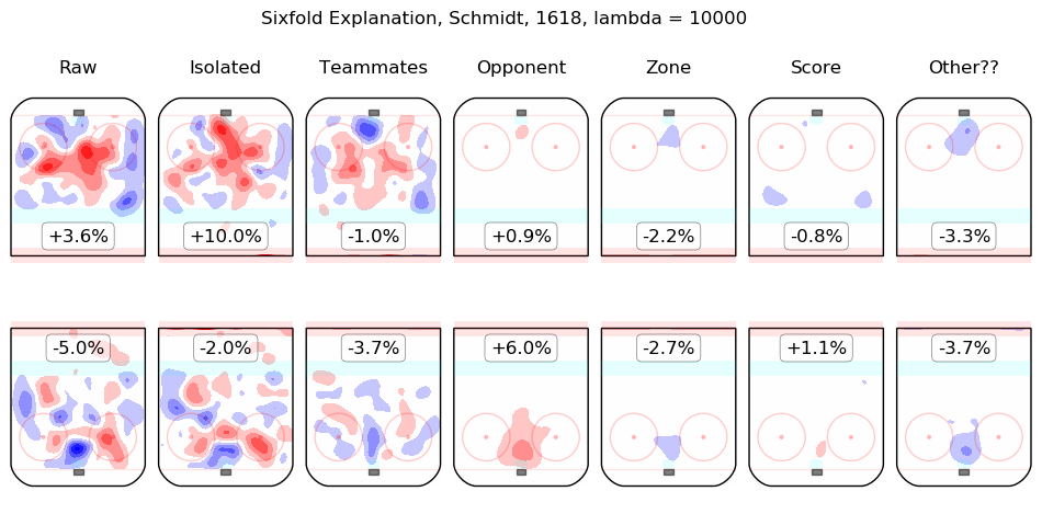
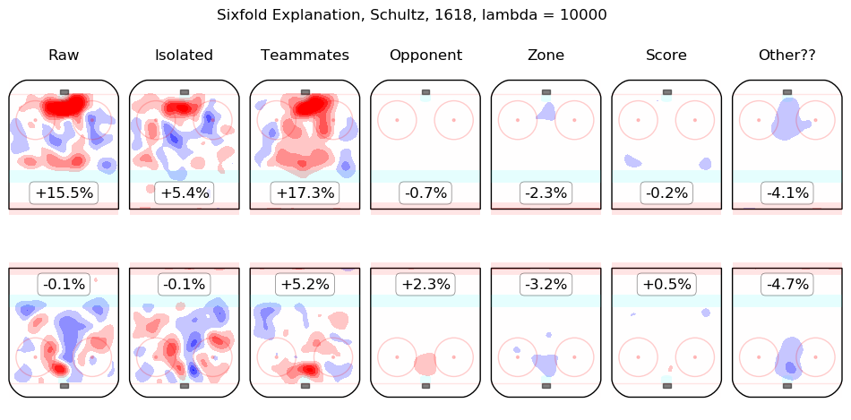
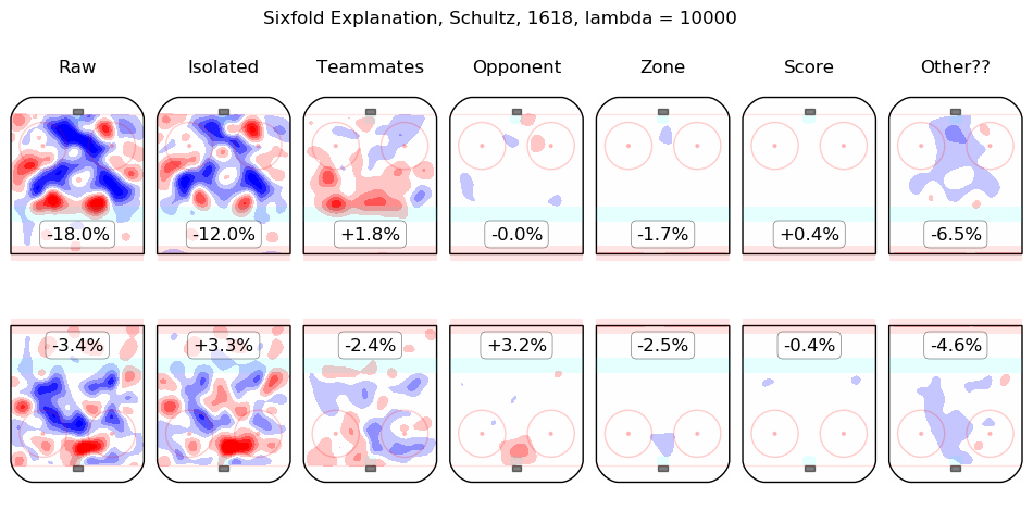
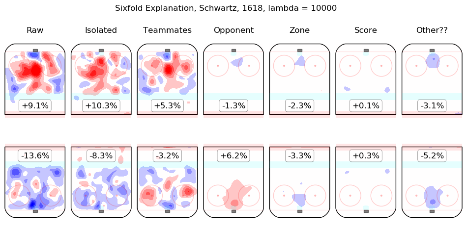
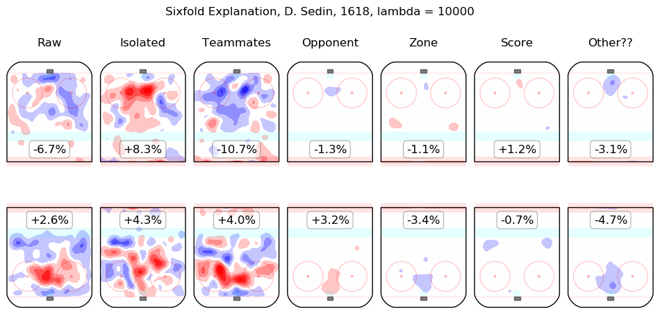
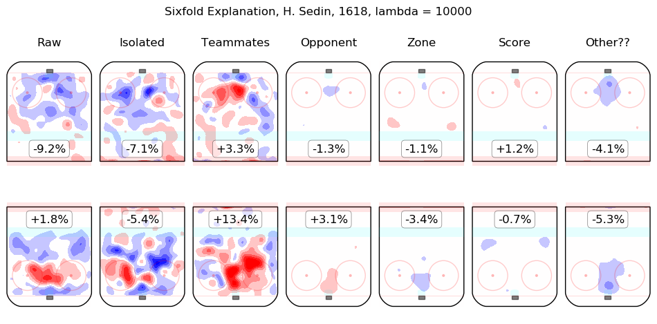
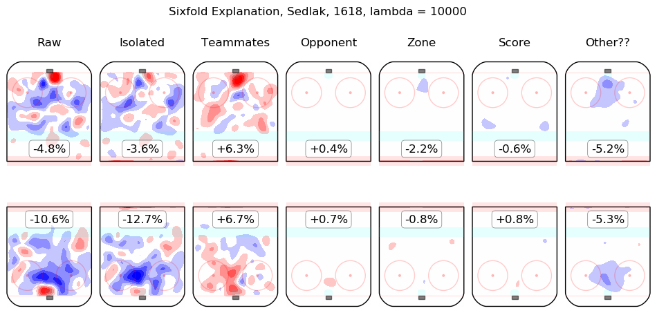
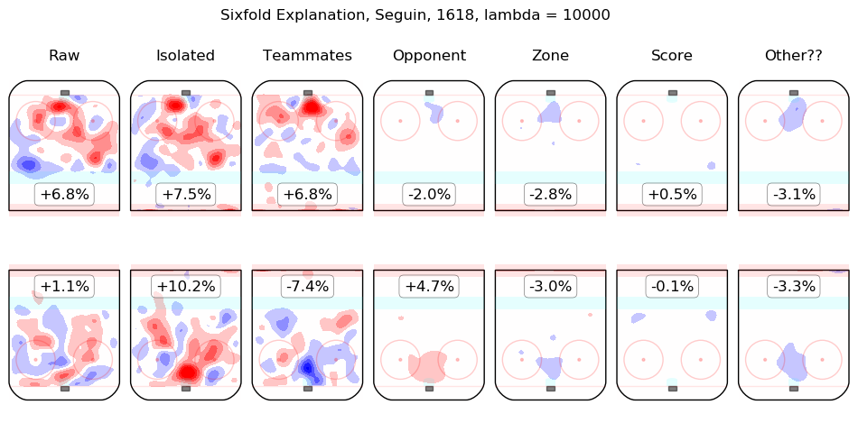
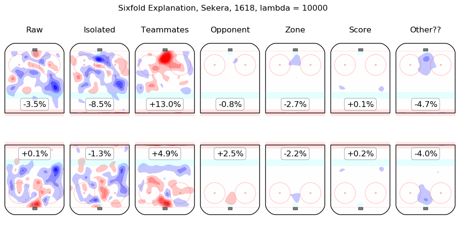
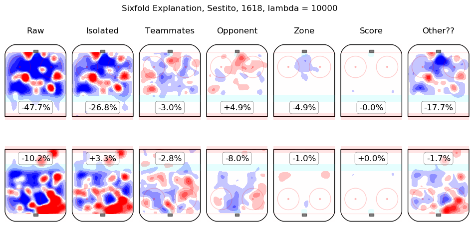
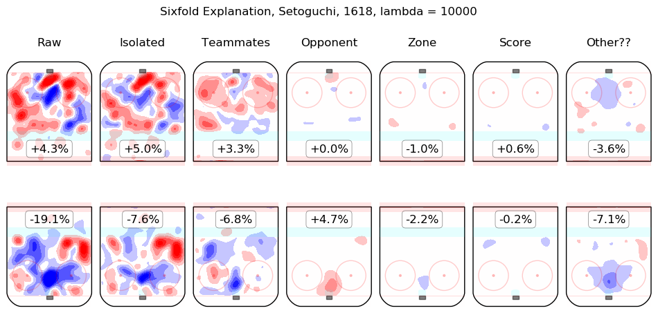
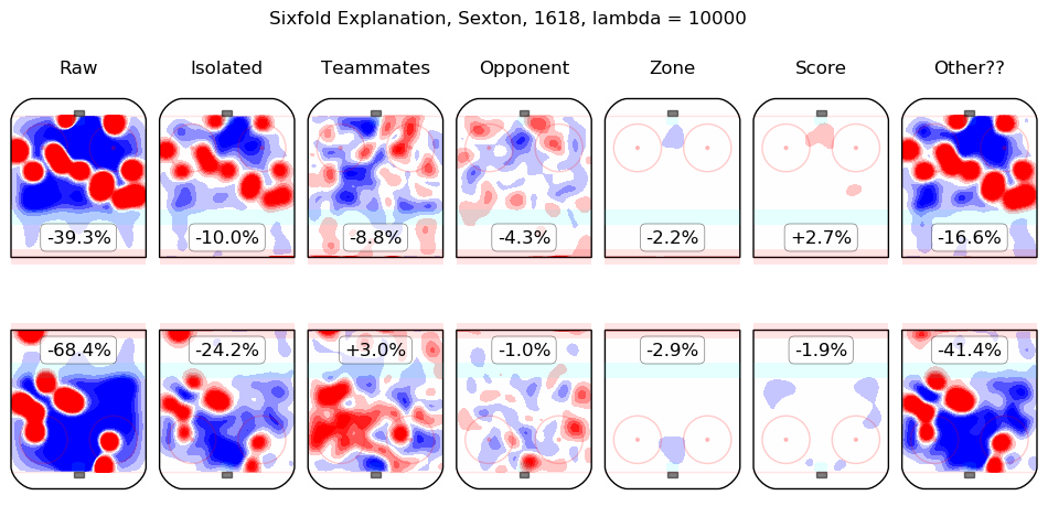
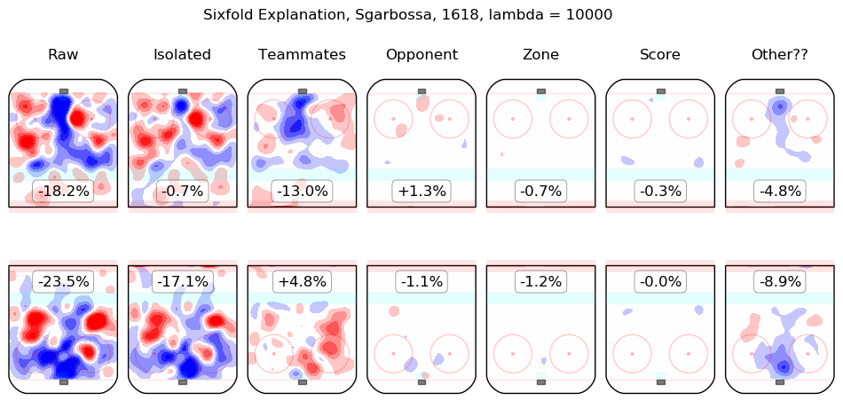
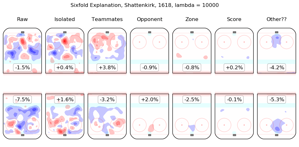
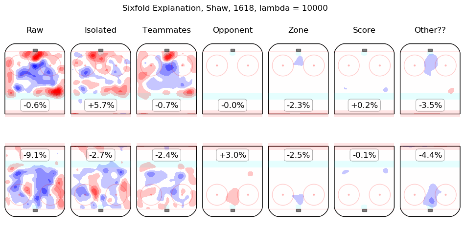
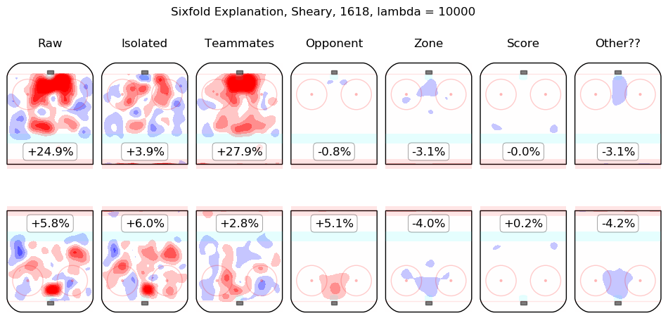
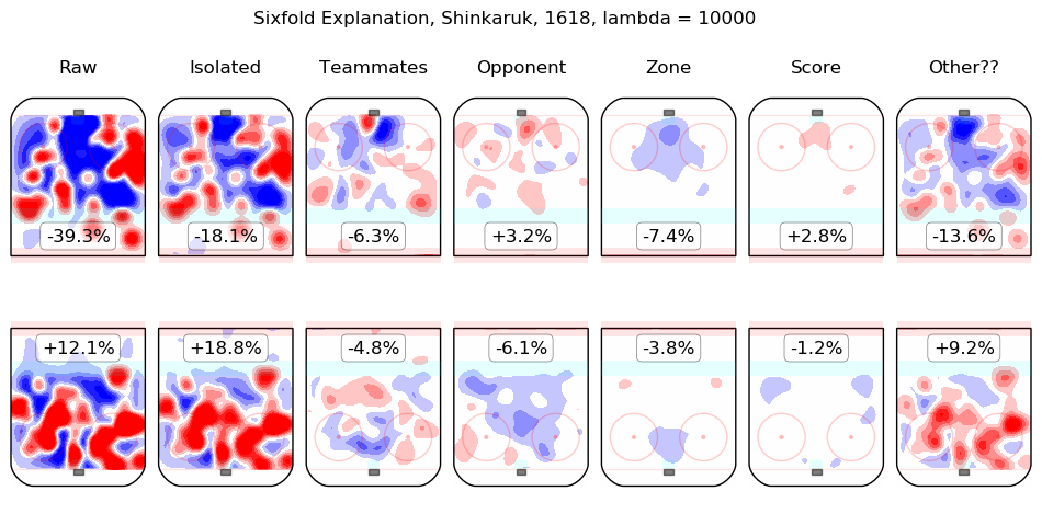
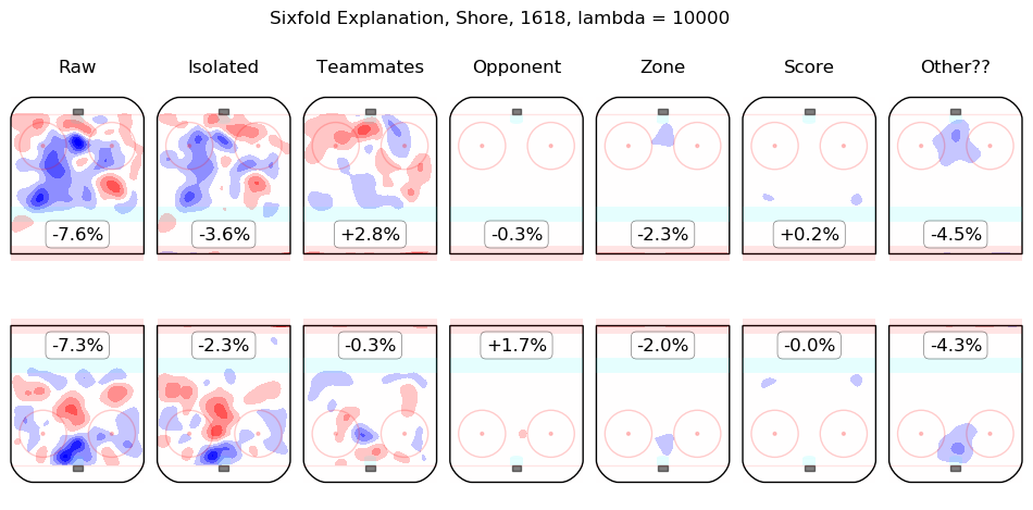
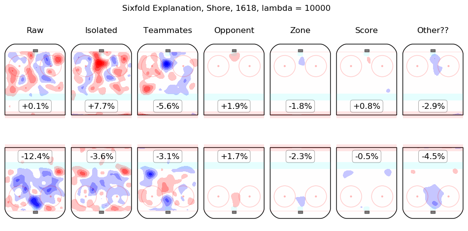
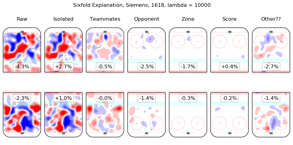
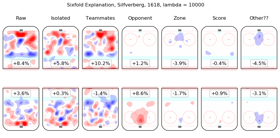
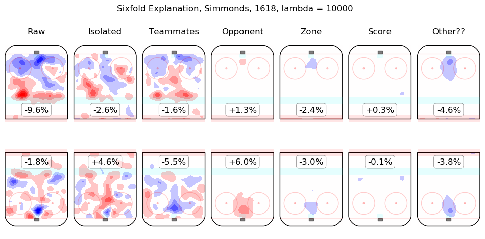
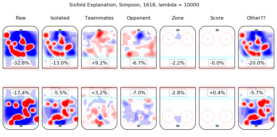
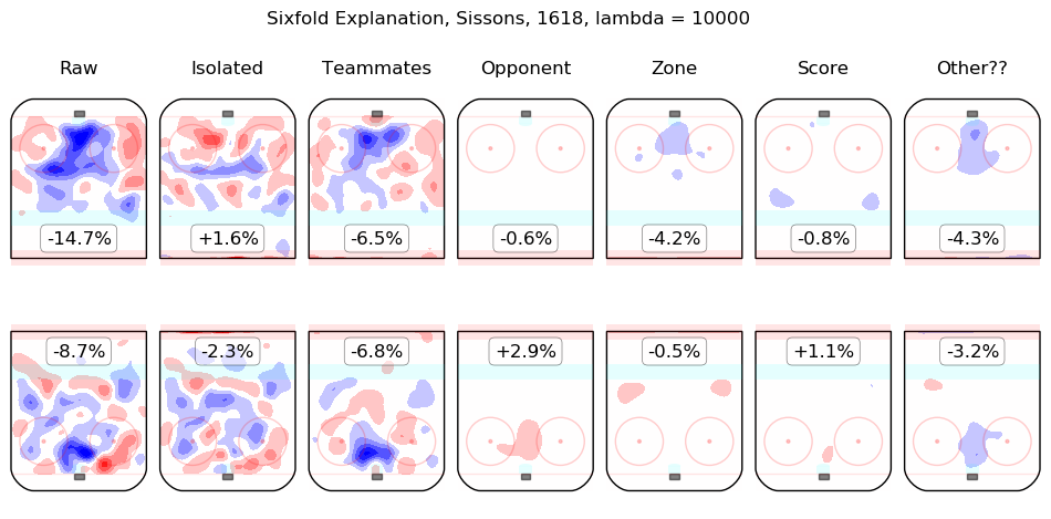
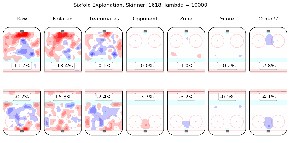
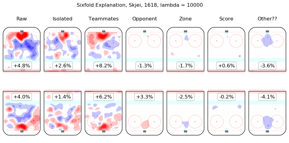
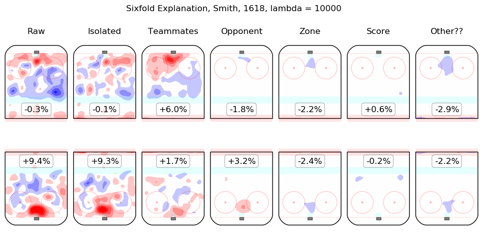
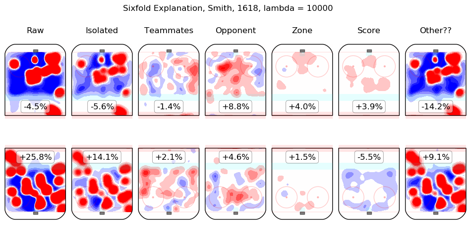
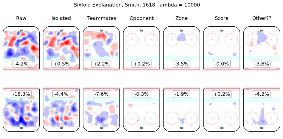
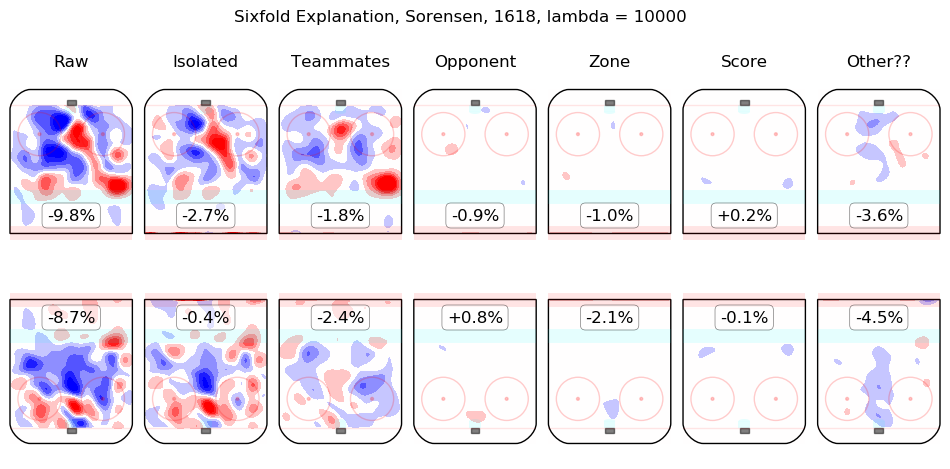
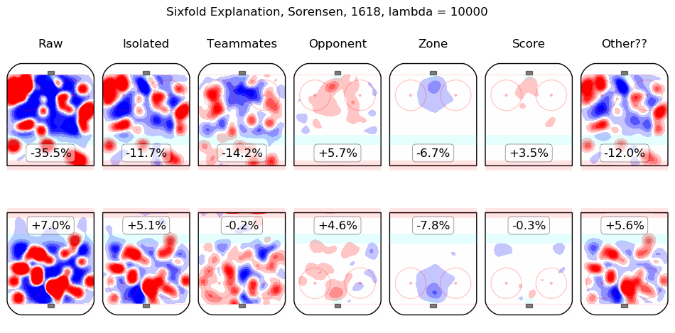
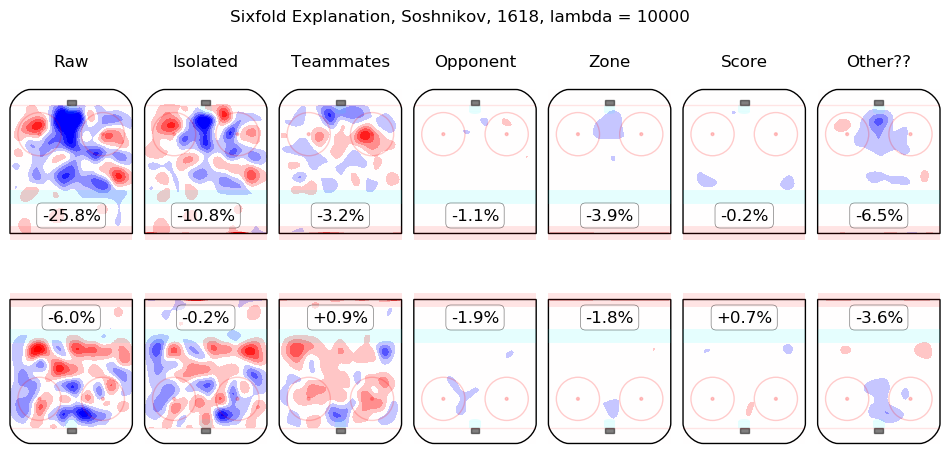
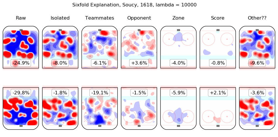
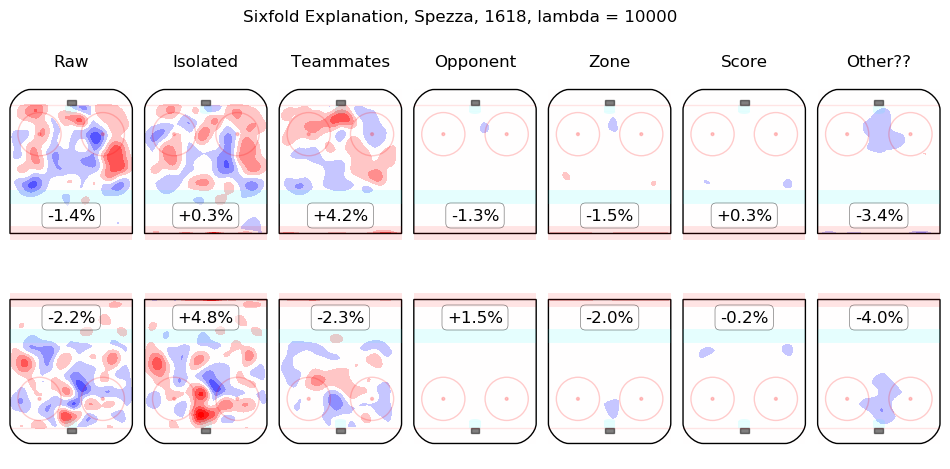
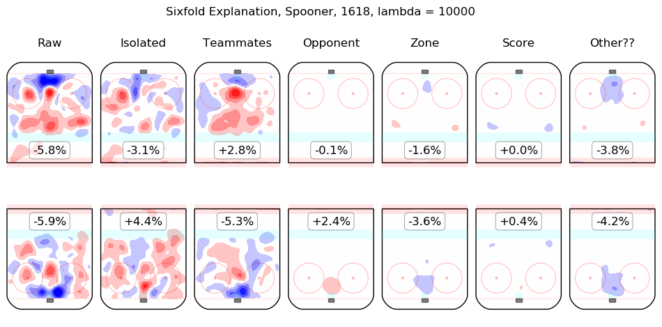
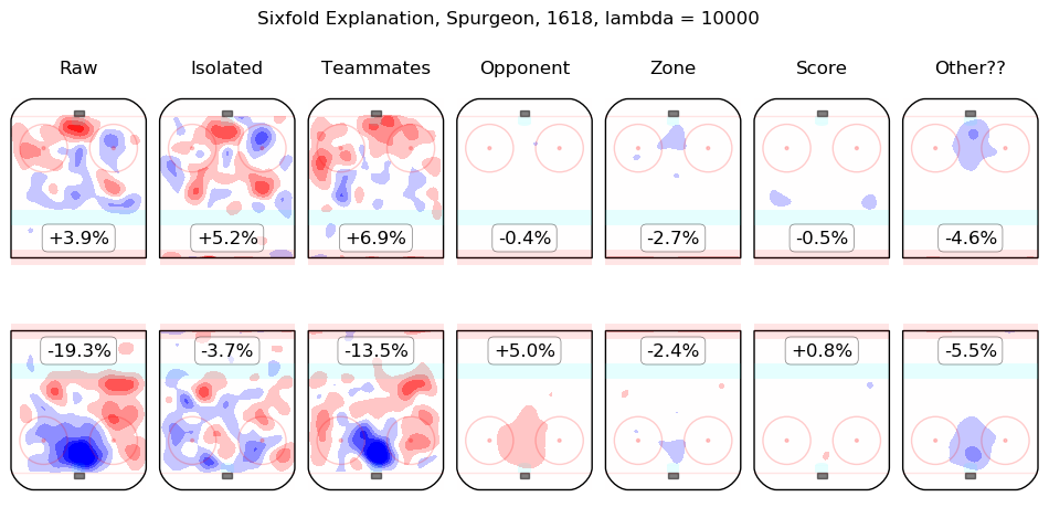
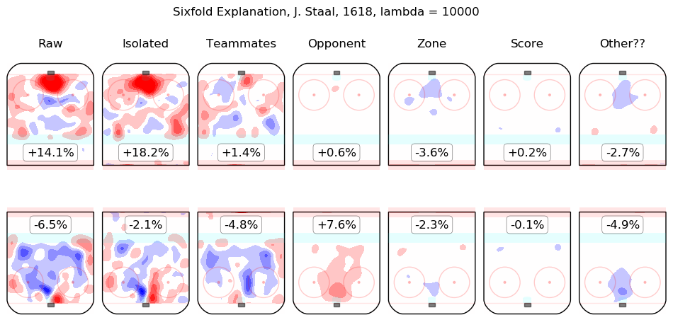
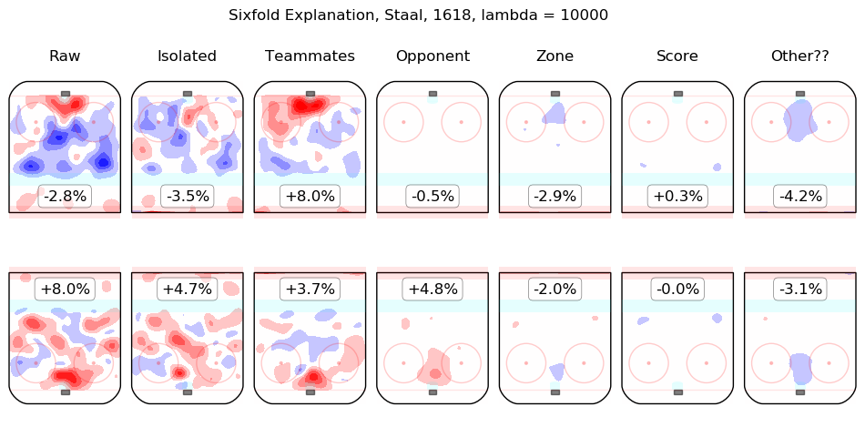
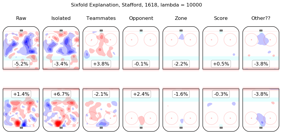
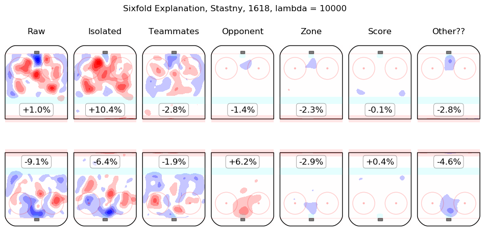
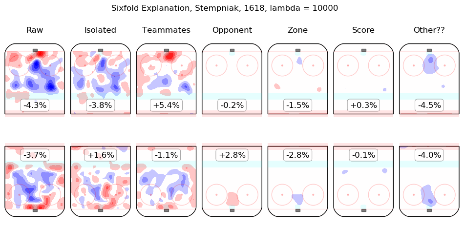
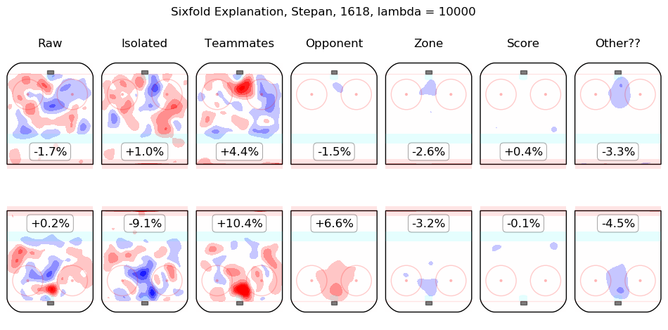
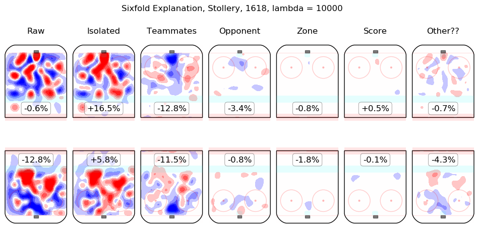
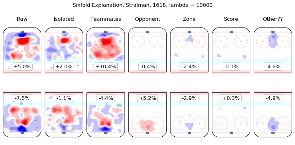
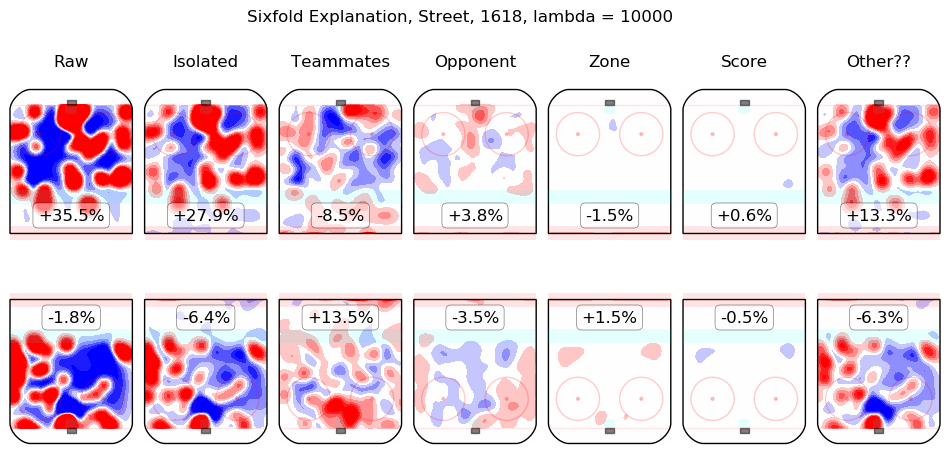
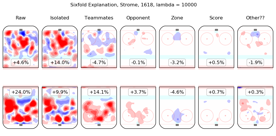
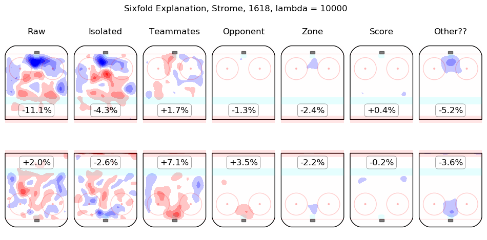
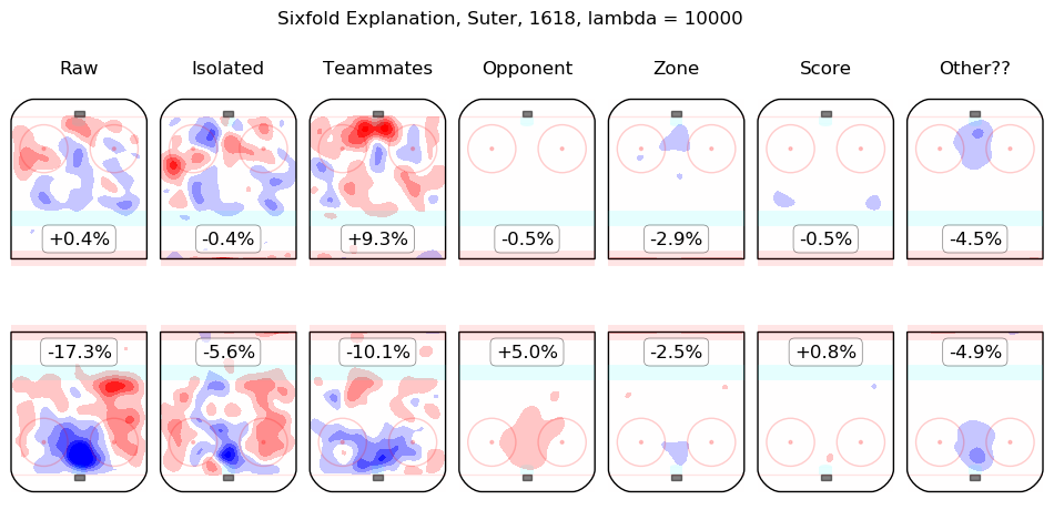
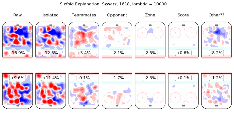
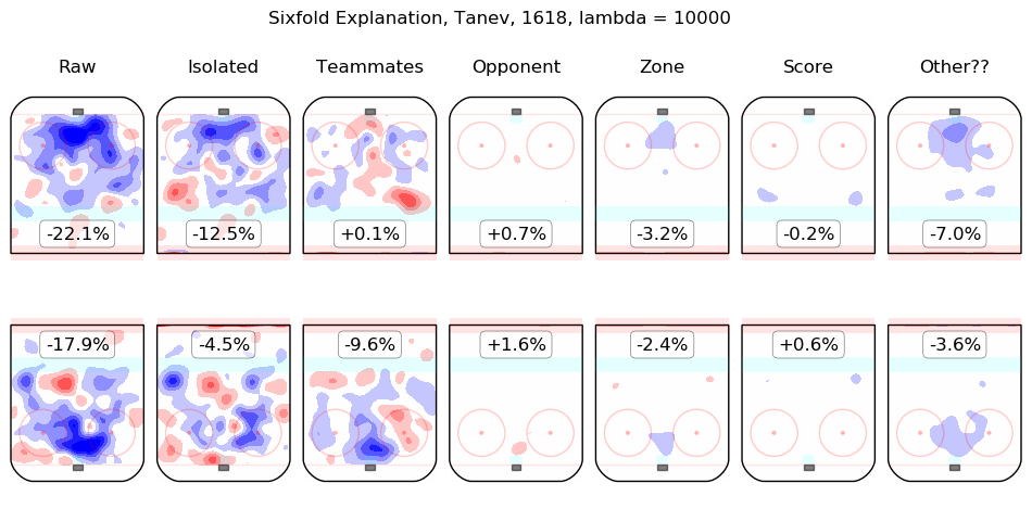
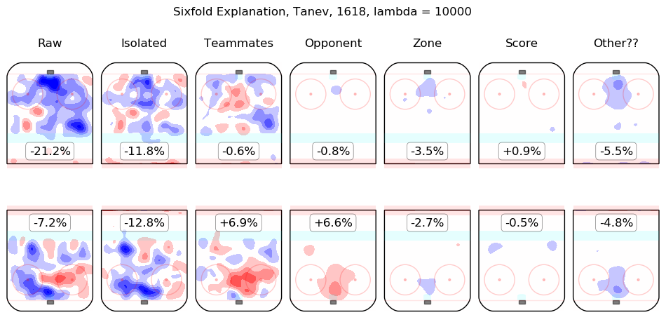
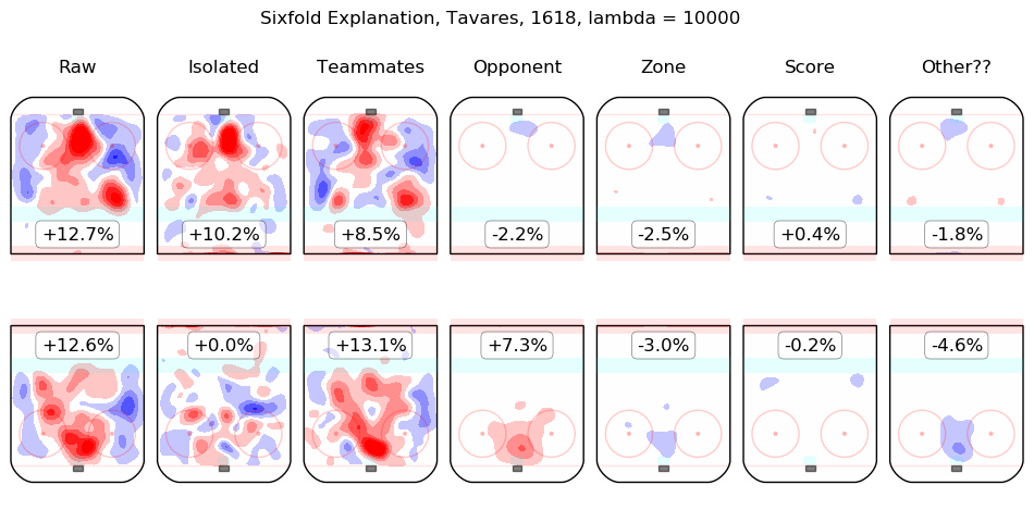
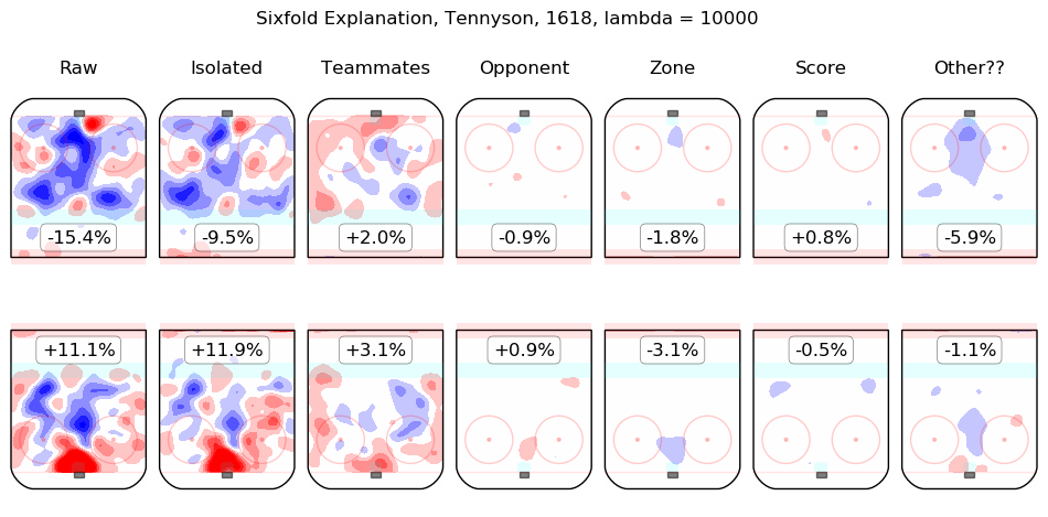
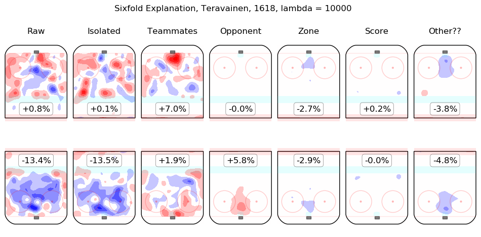
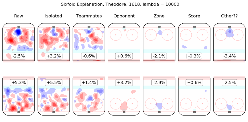
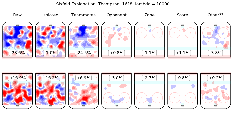
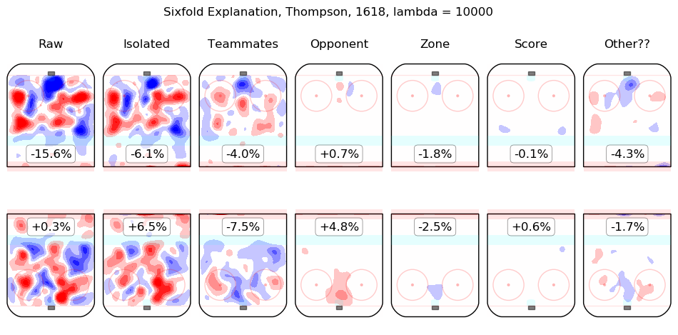
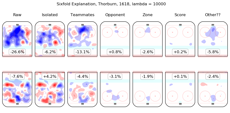
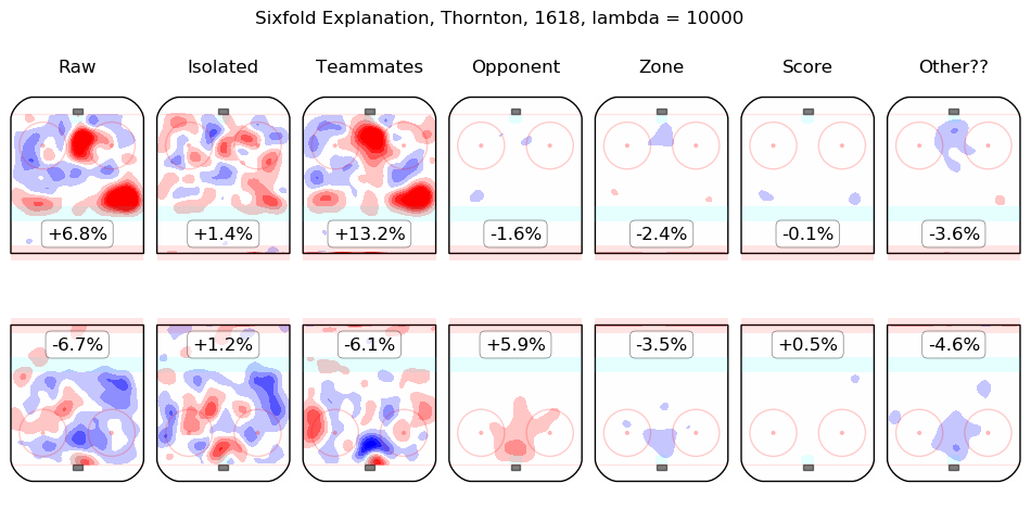
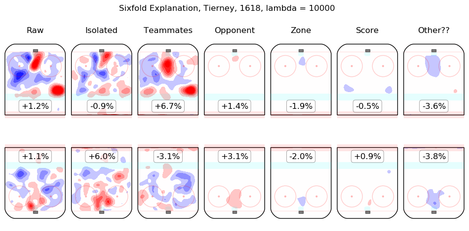
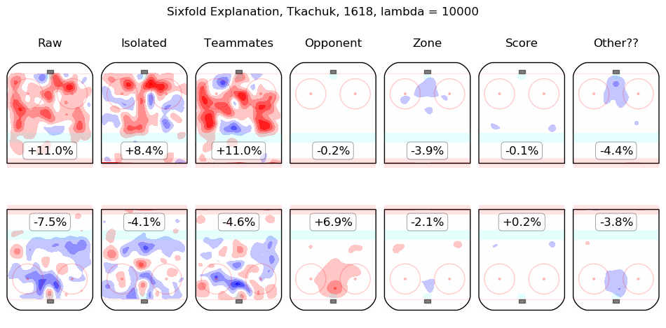
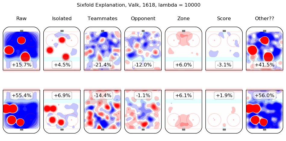
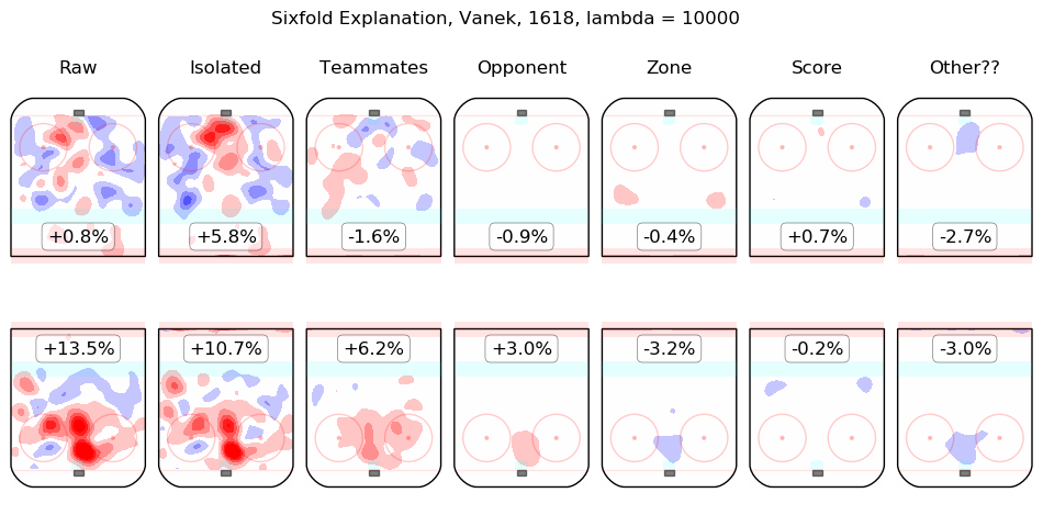
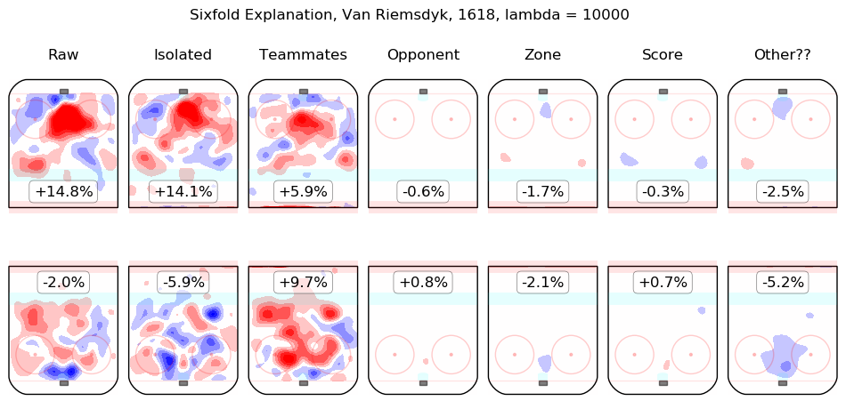
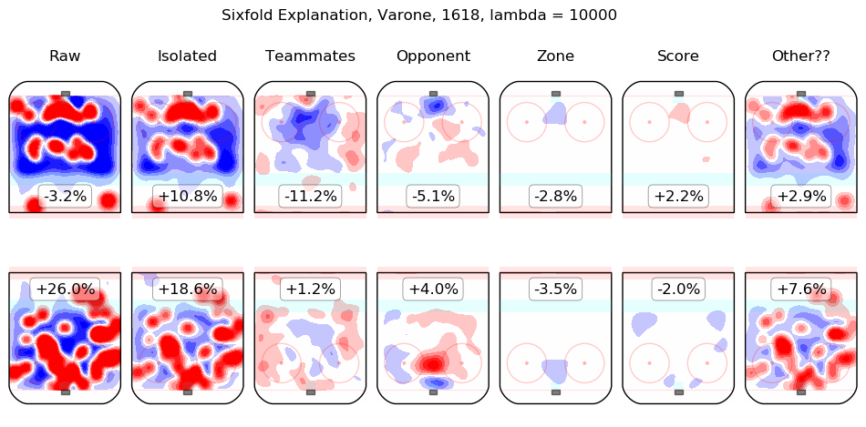
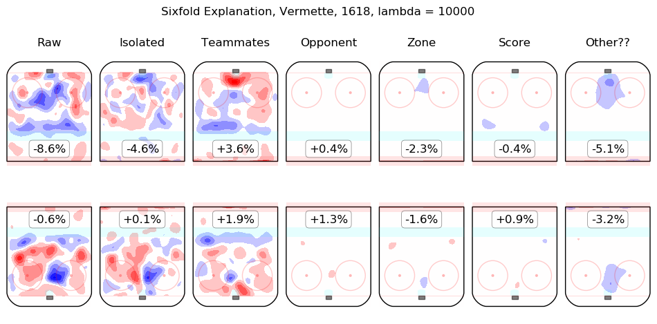
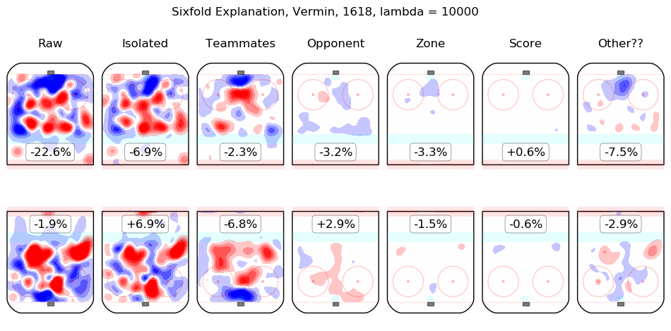
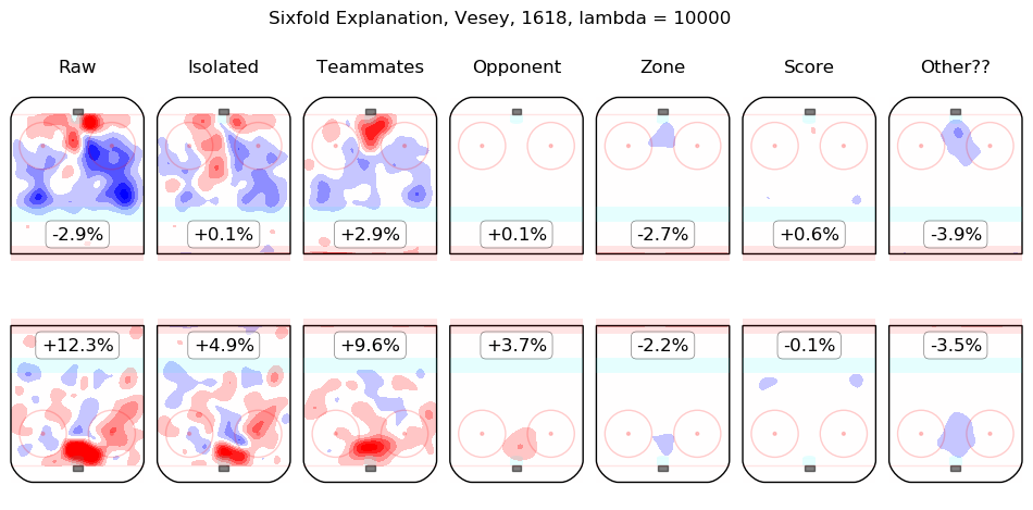
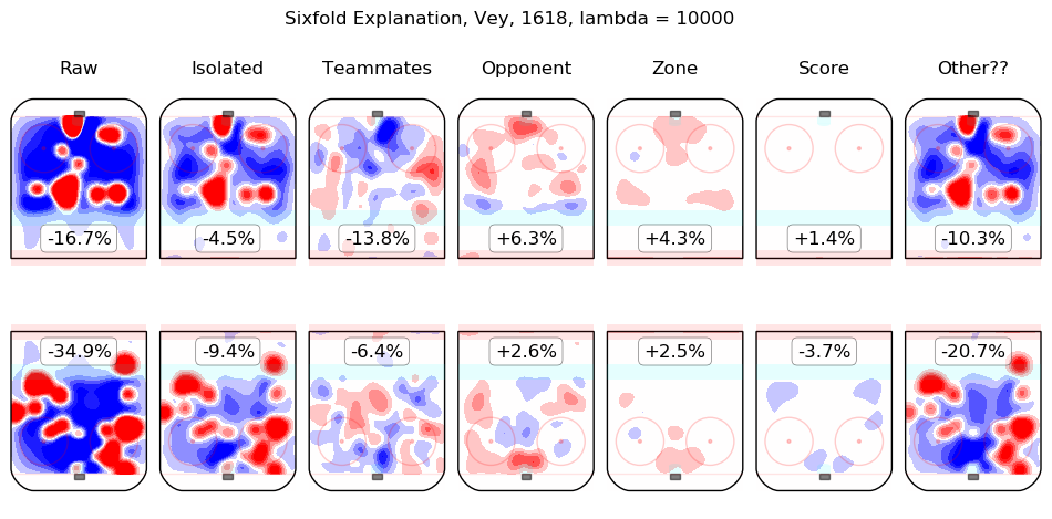
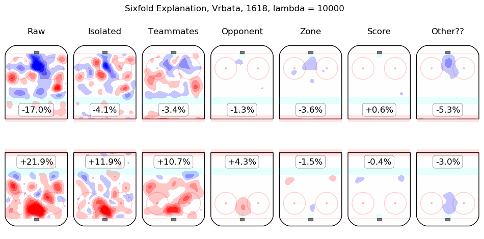
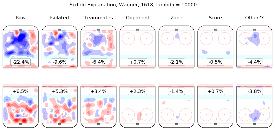
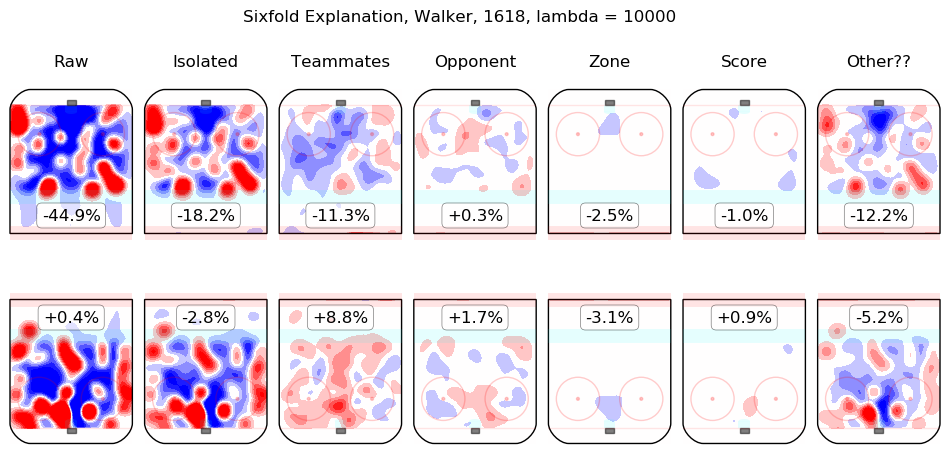
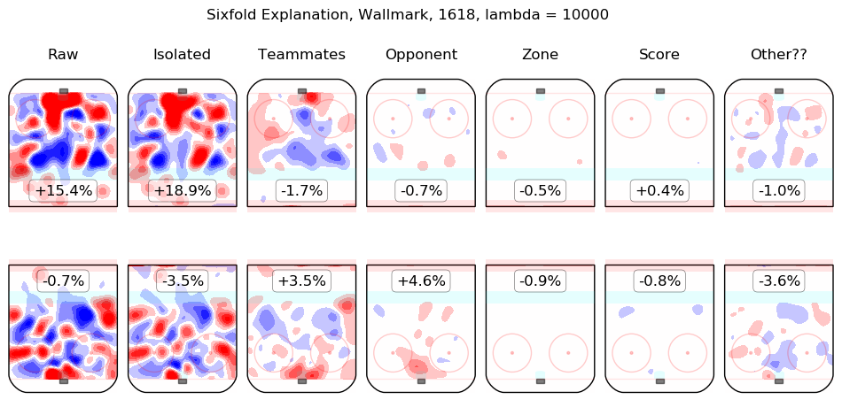
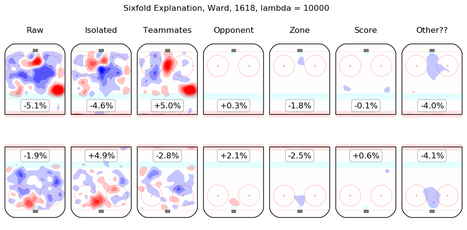
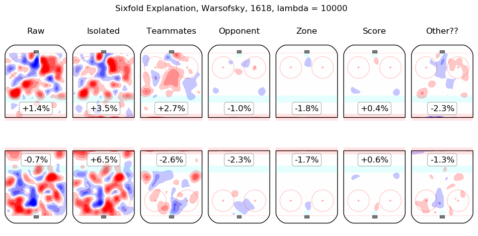
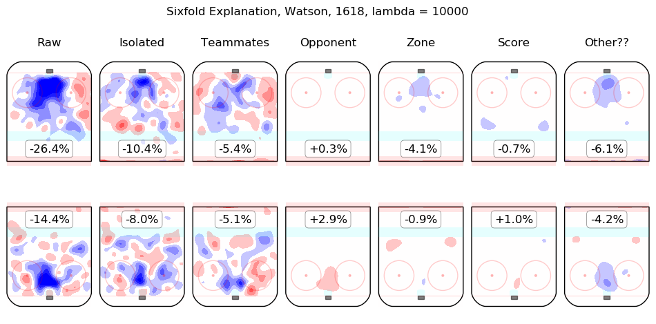
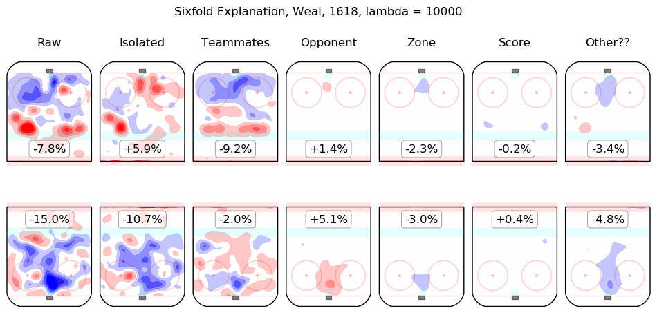
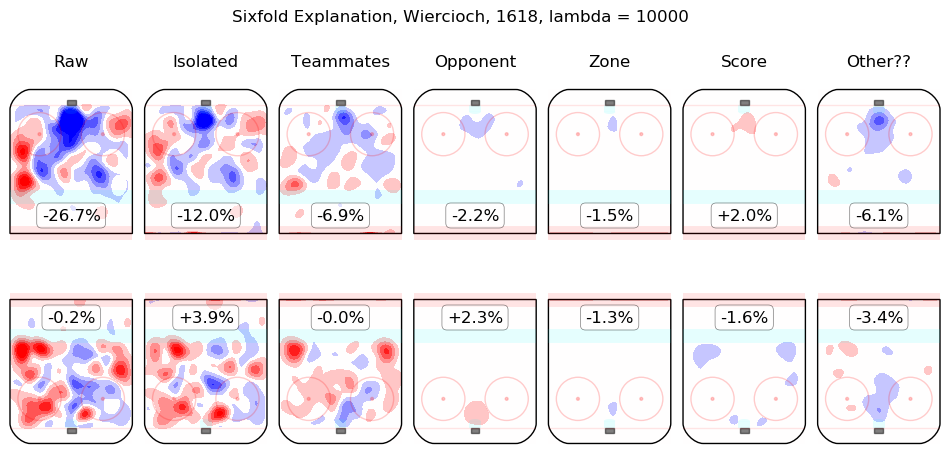
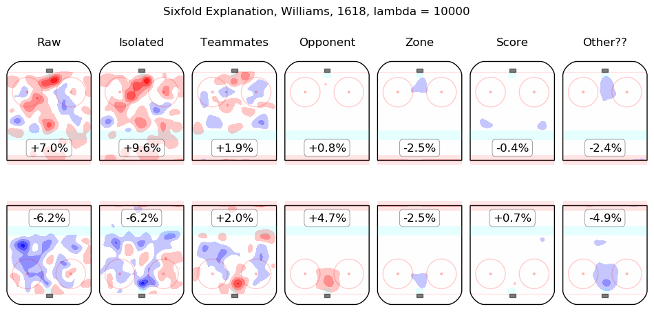
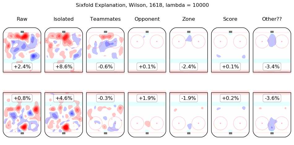
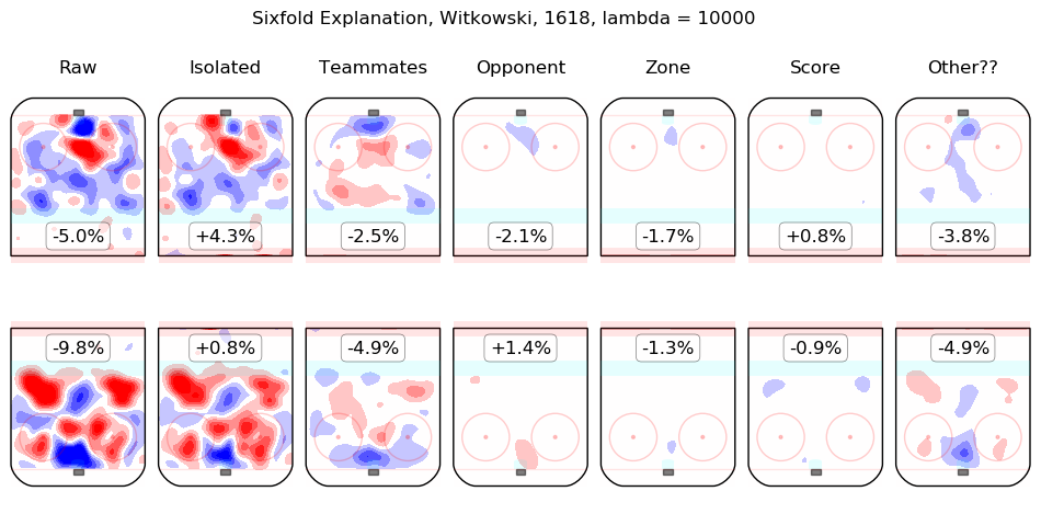
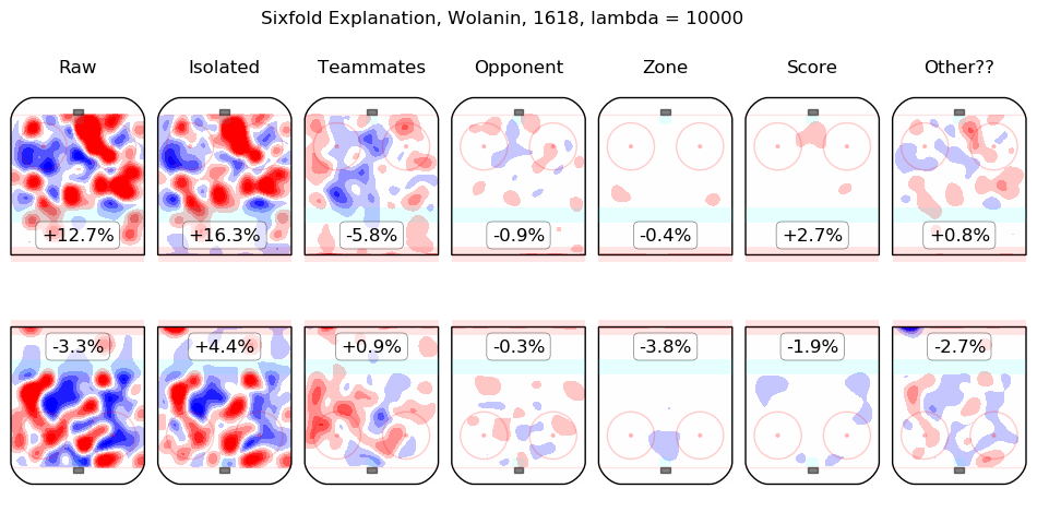
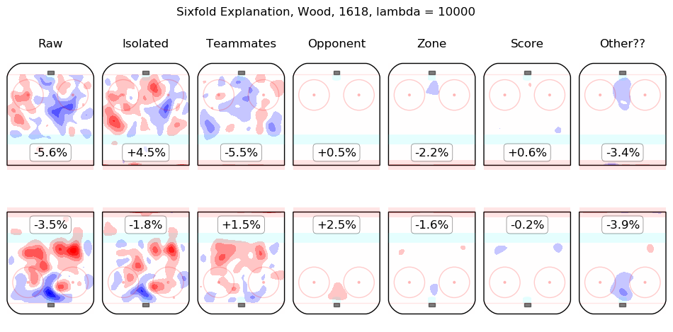
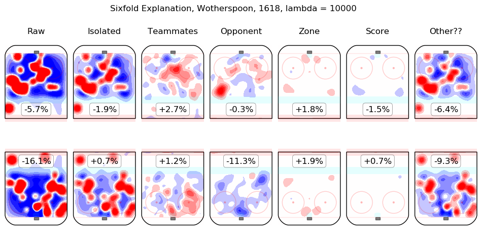
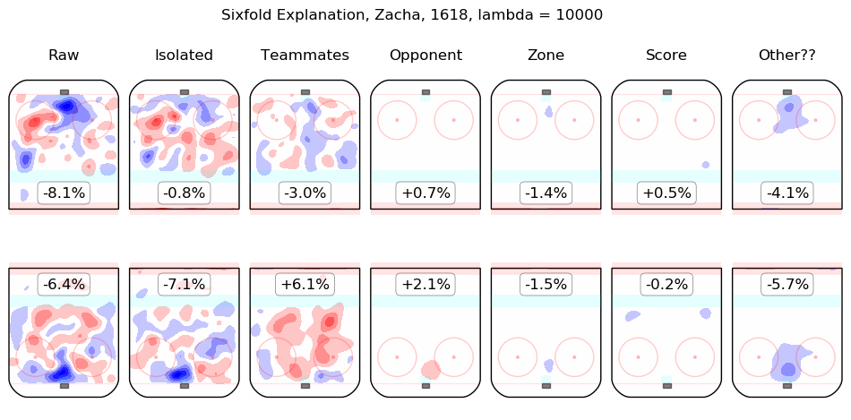
Results Appendix
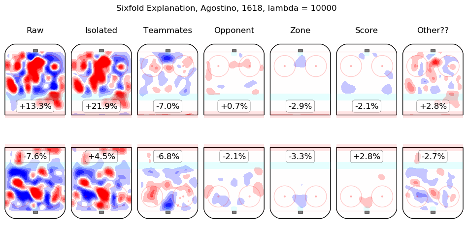
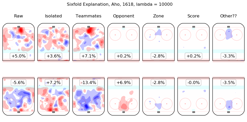
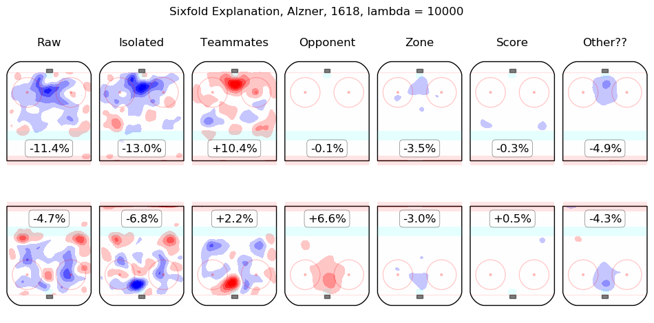
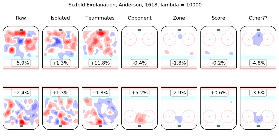
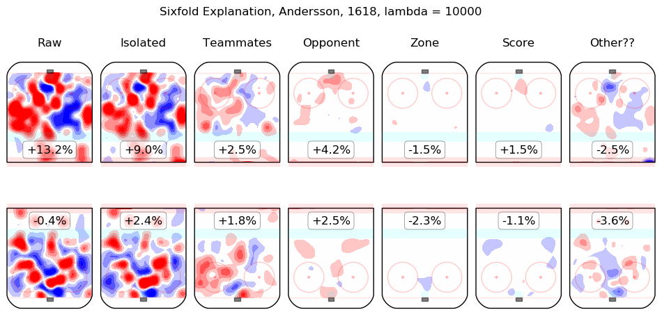
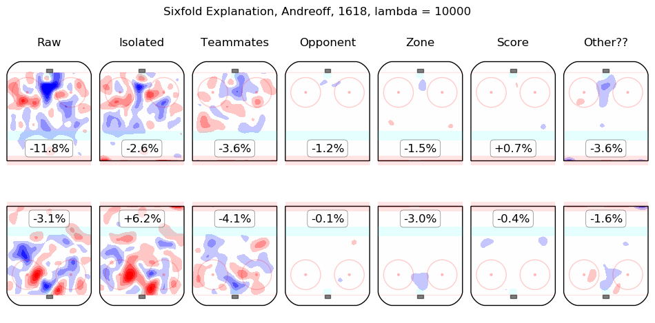
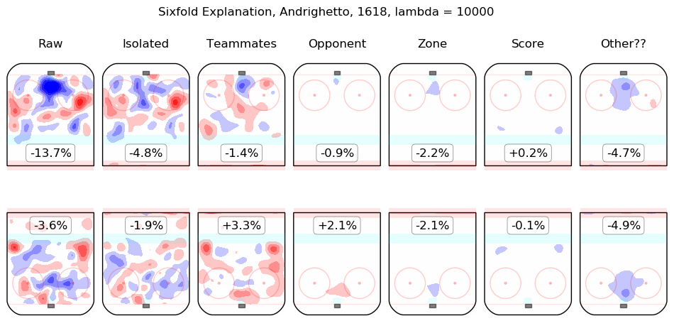
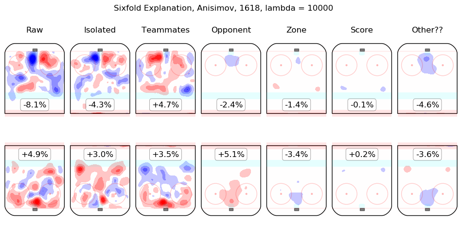
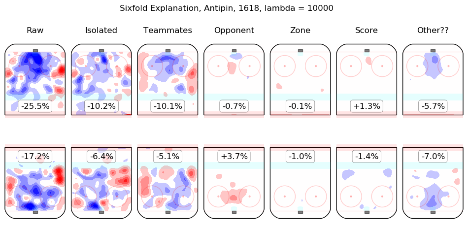
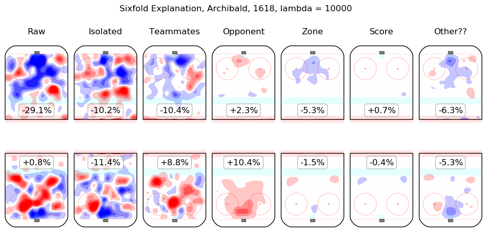
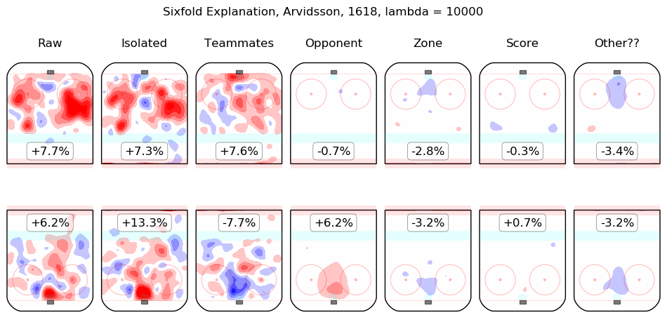
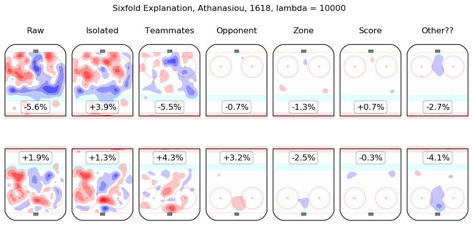
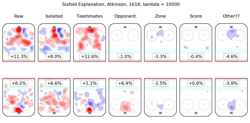
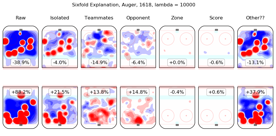
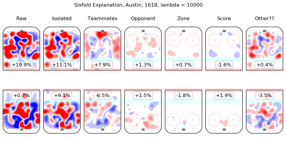
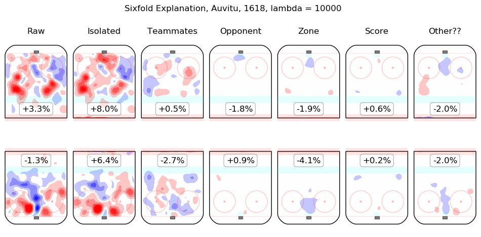
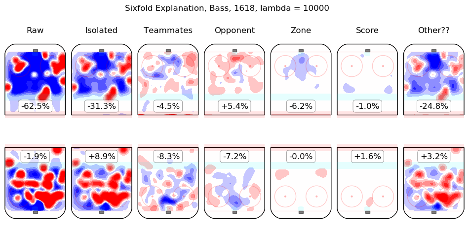
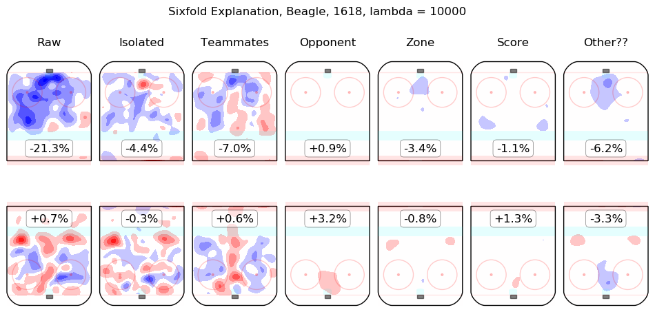
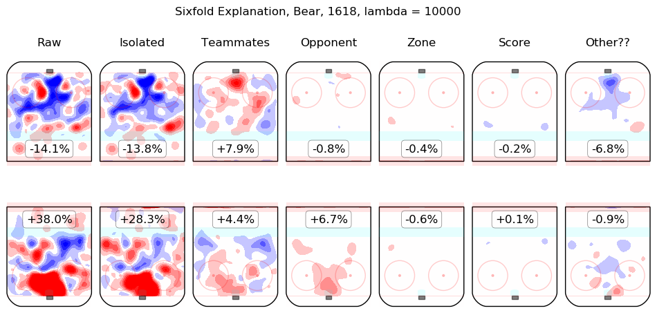
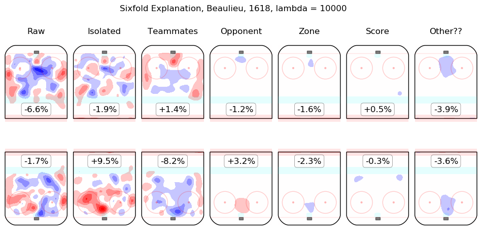
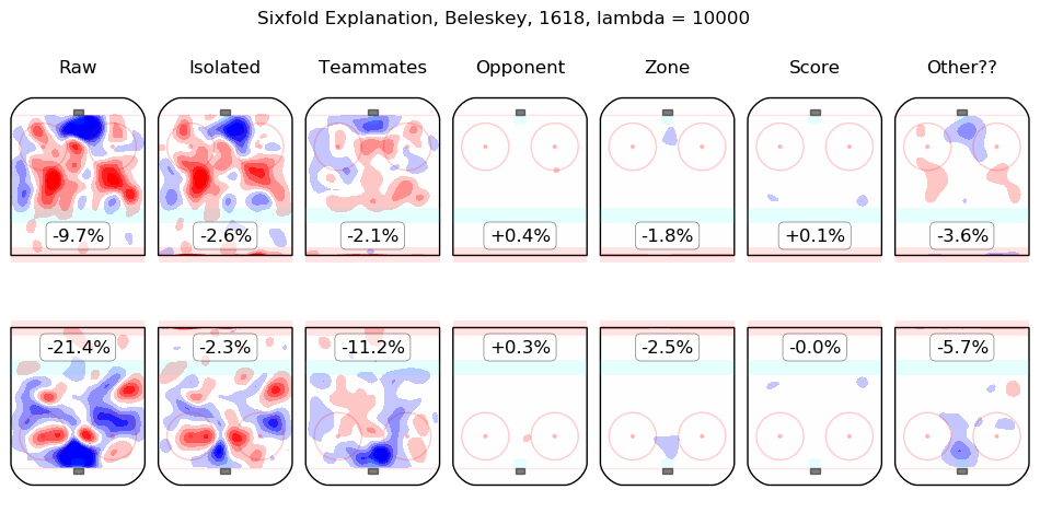
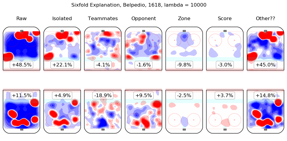
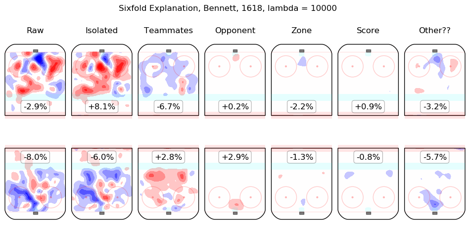
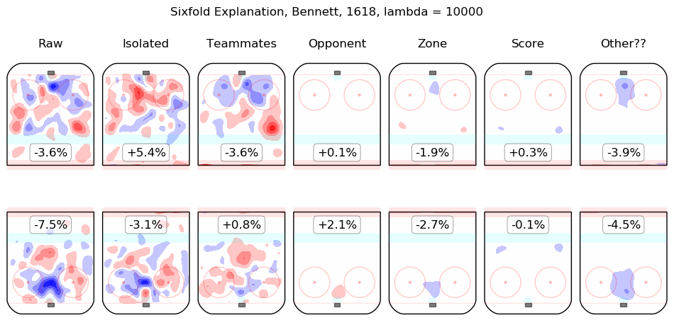
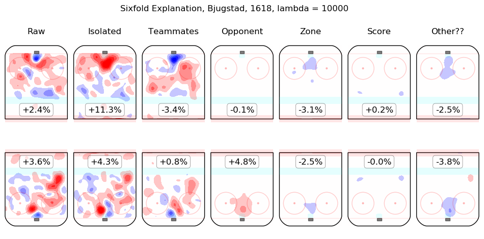
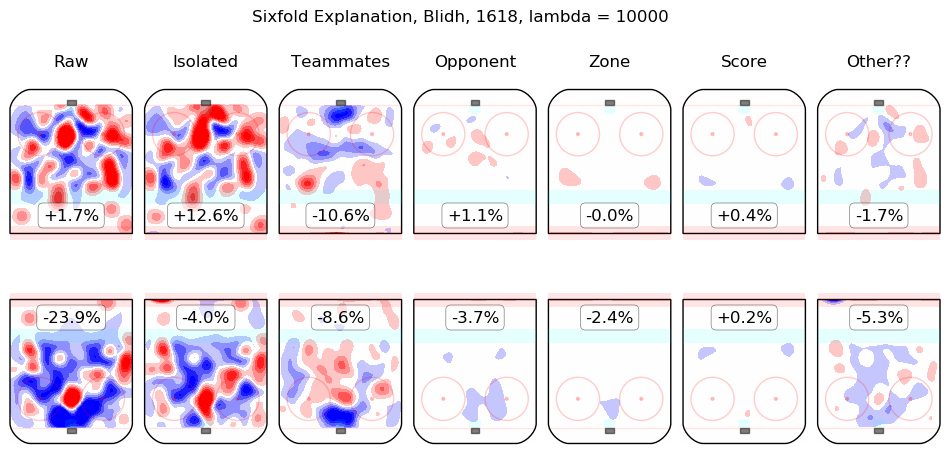
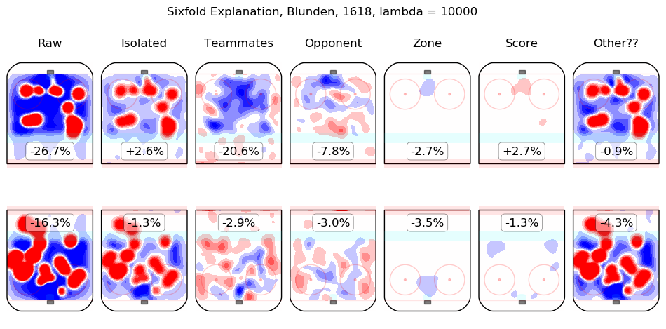
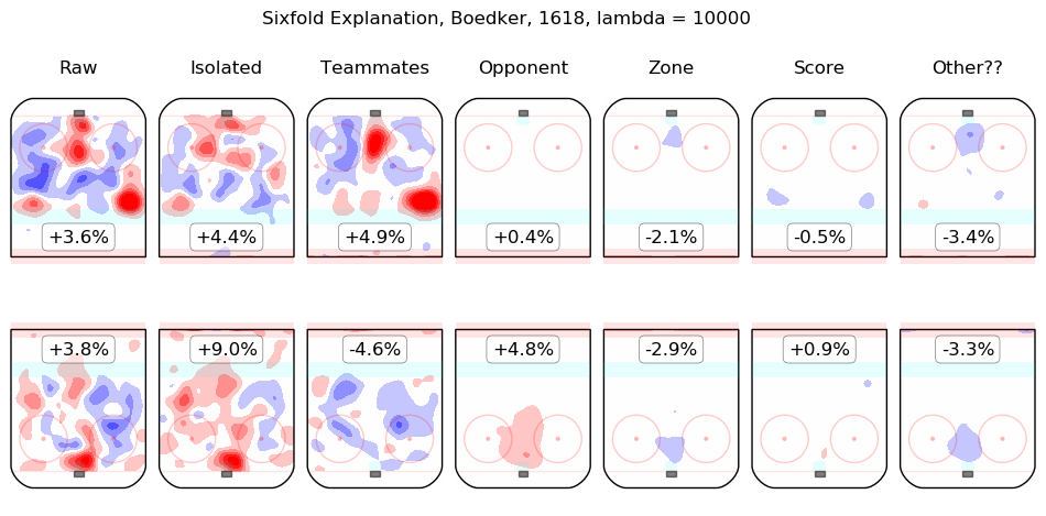
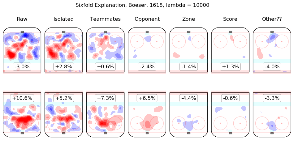
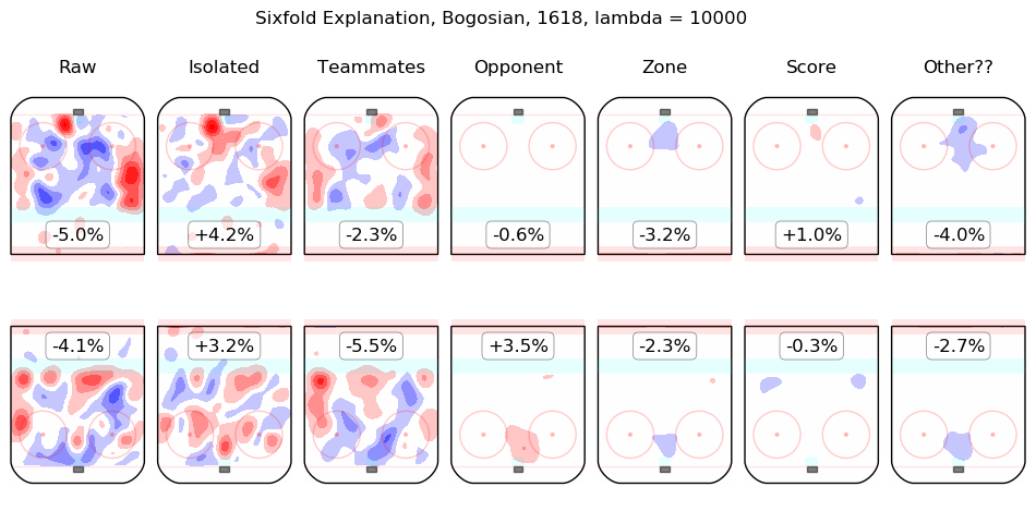
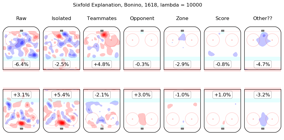
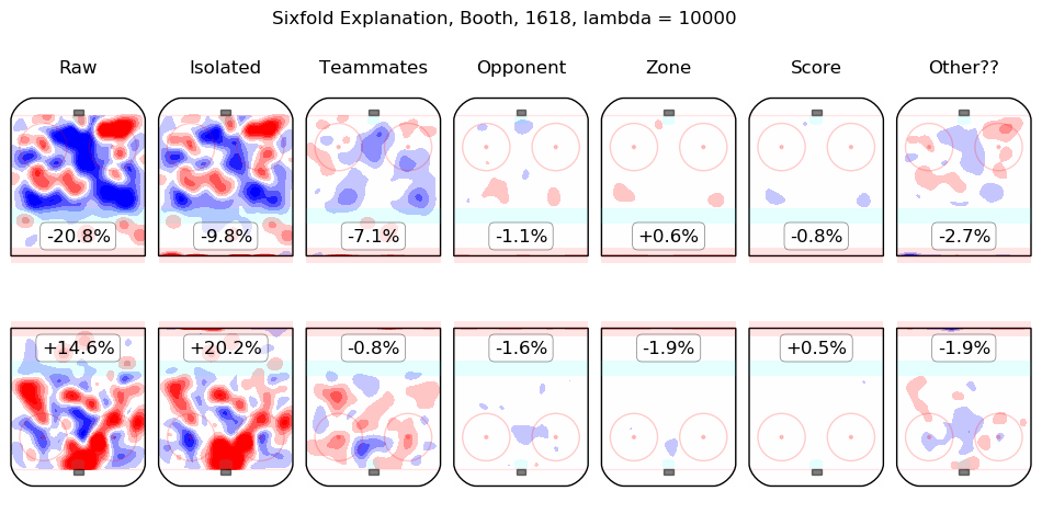
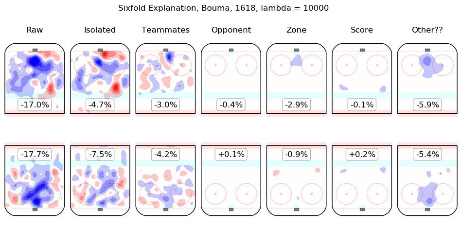
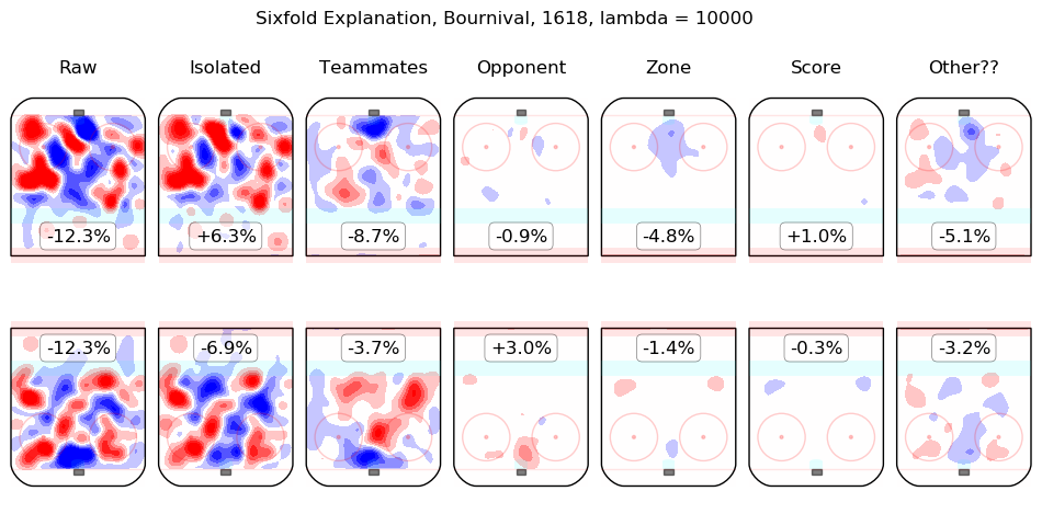
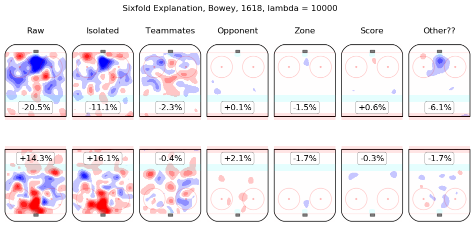
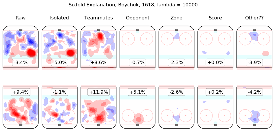
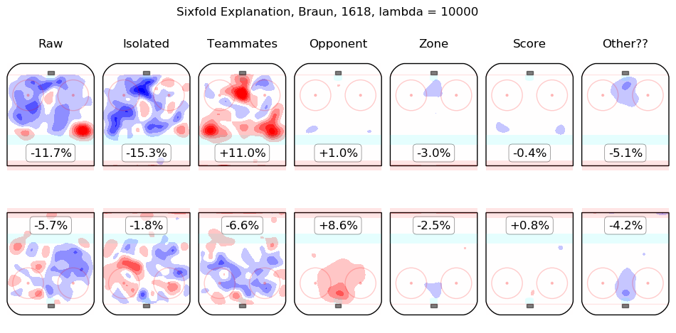
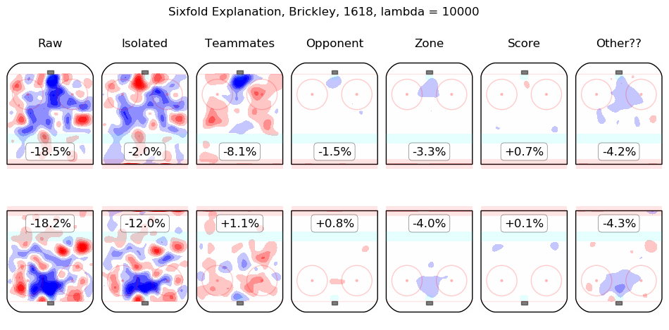
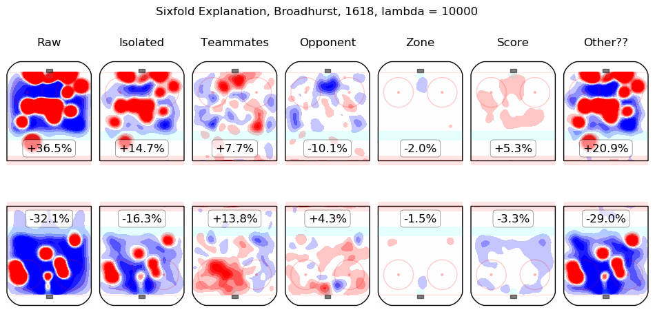
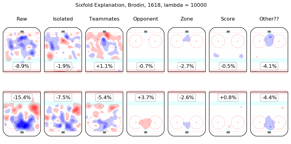
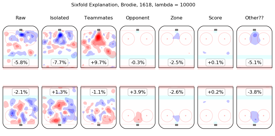
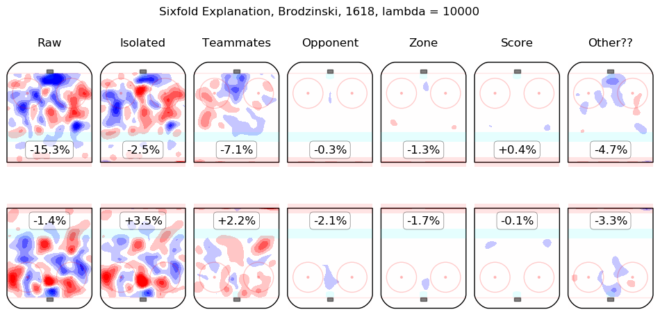
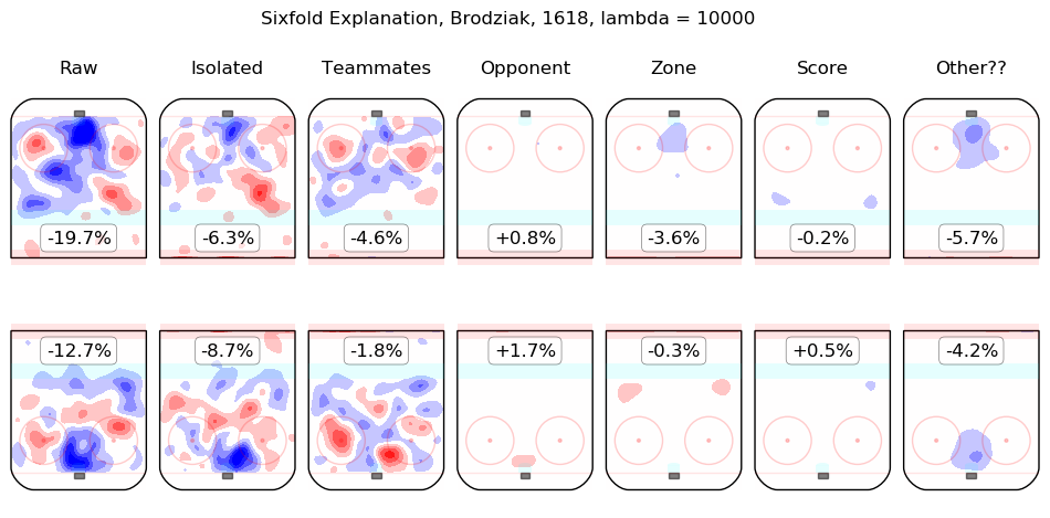
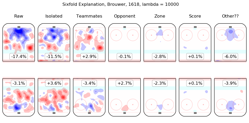
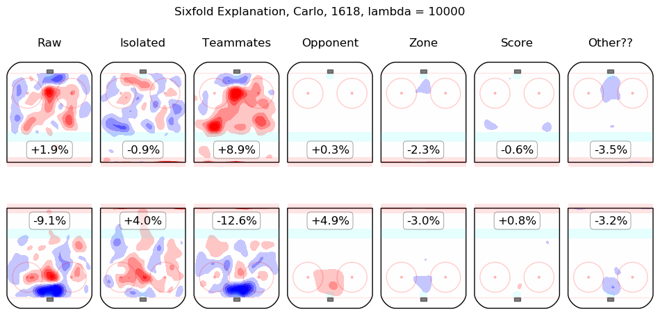
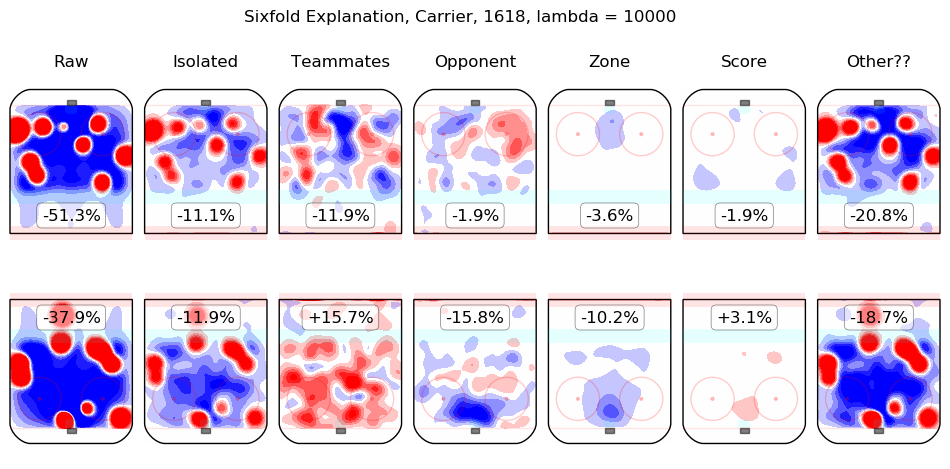
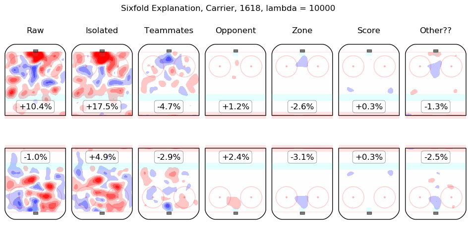
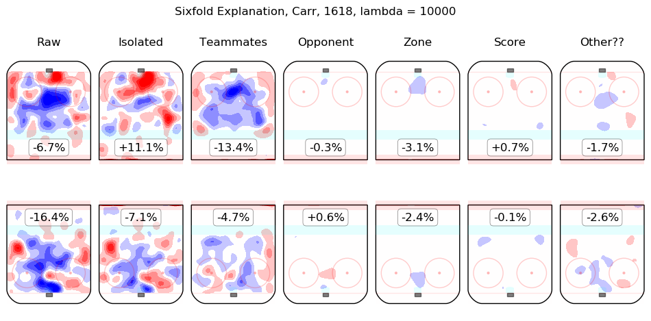
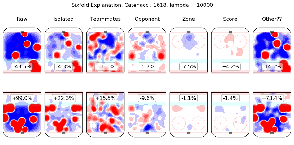
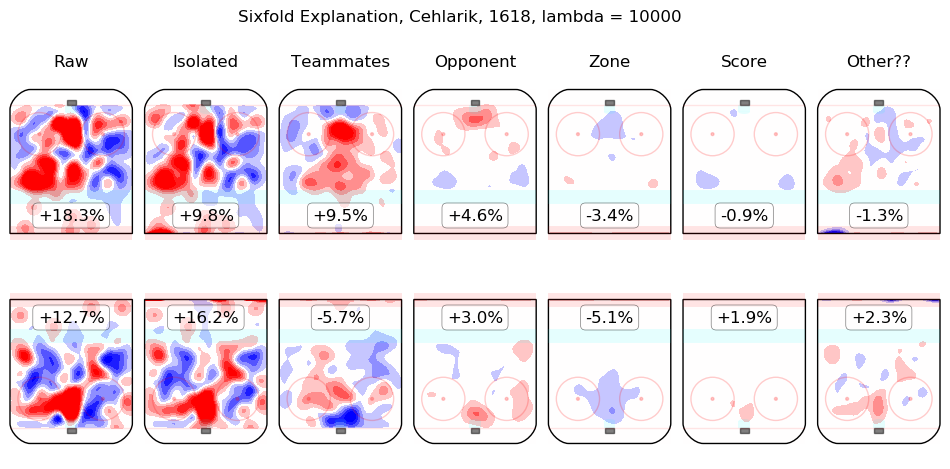
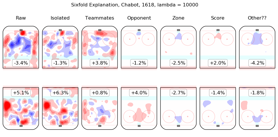
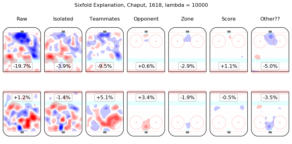
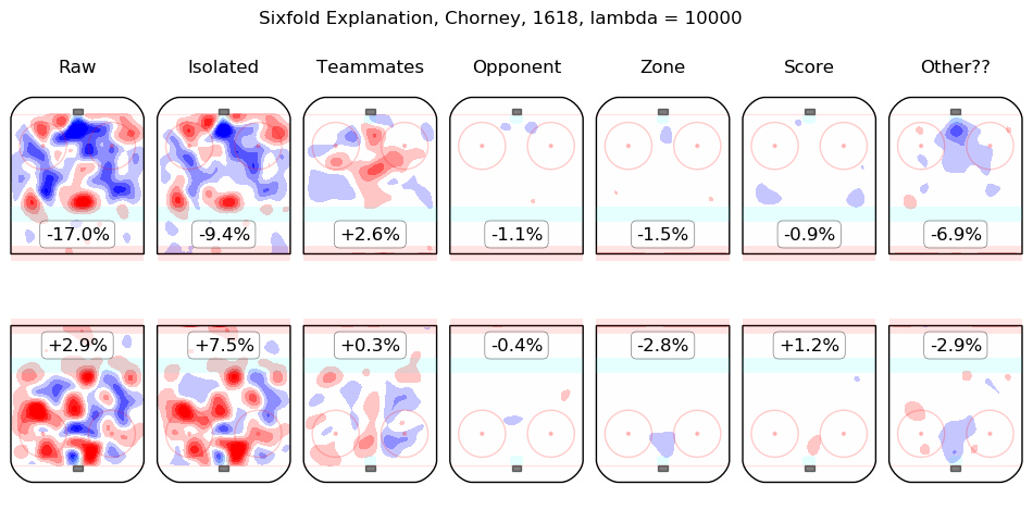
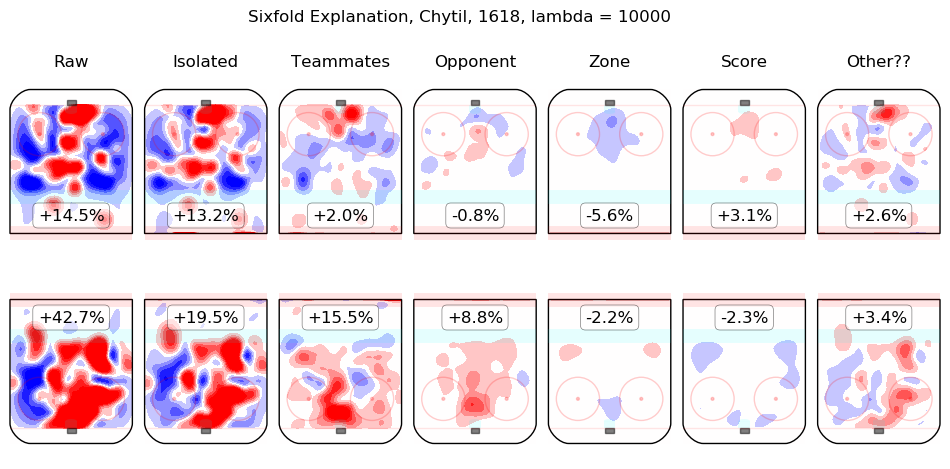
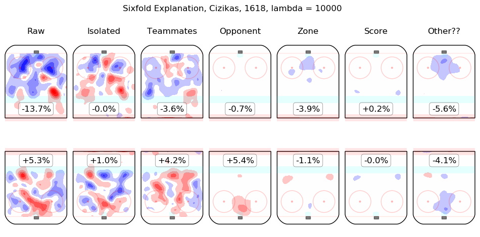
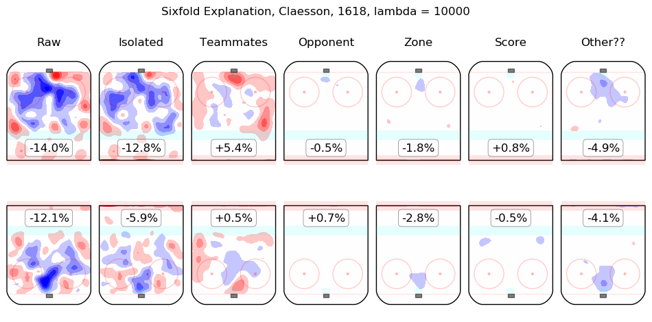
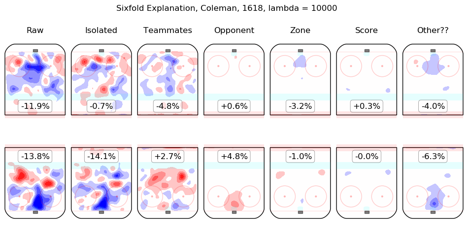
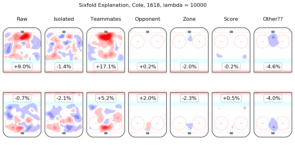
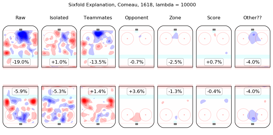
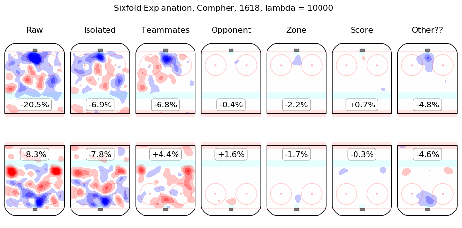
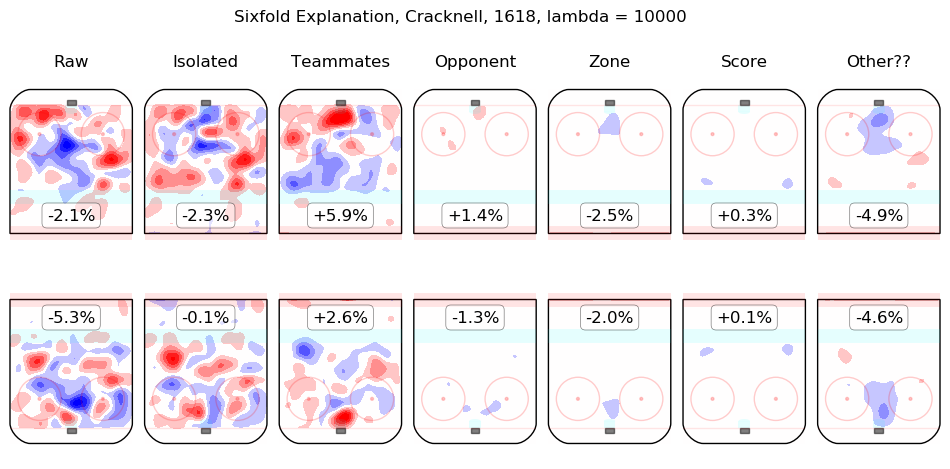
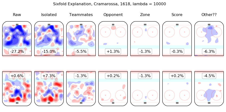
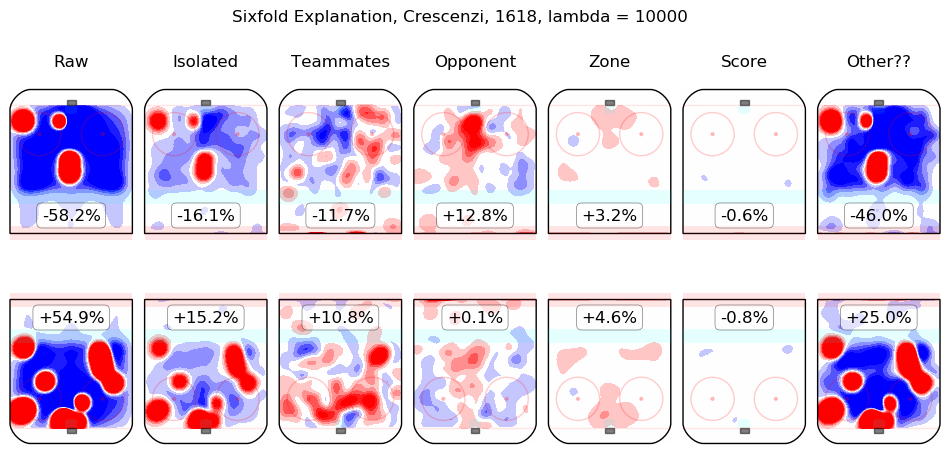
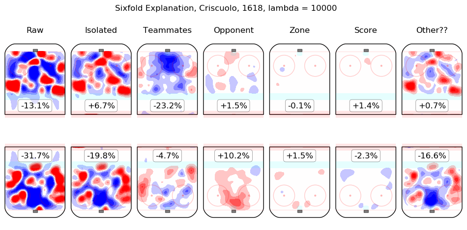
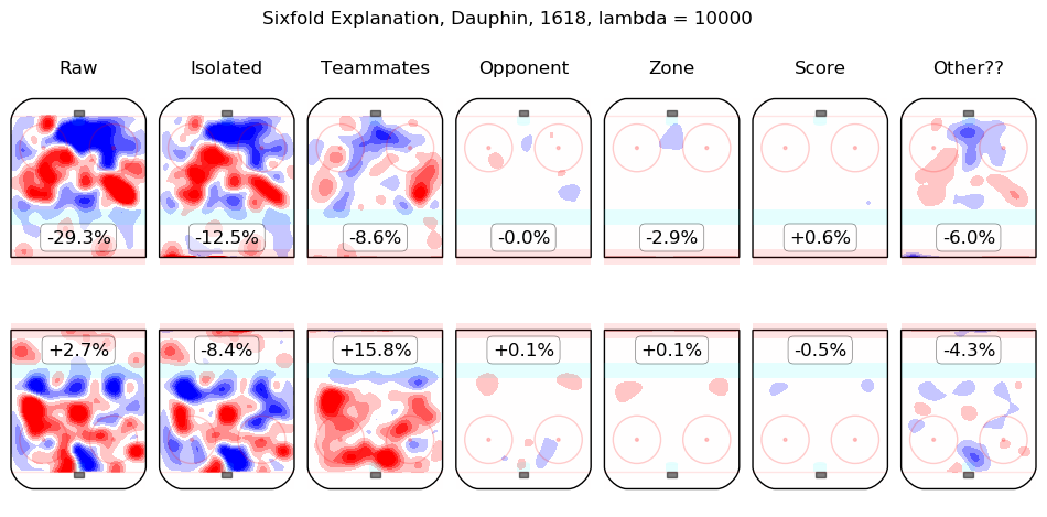
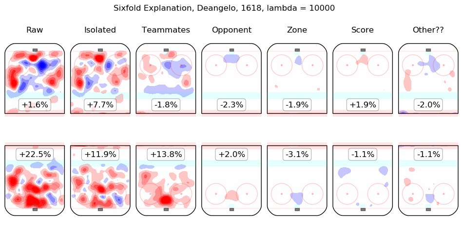
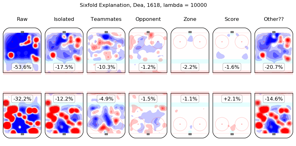
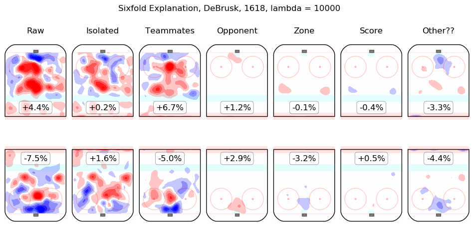
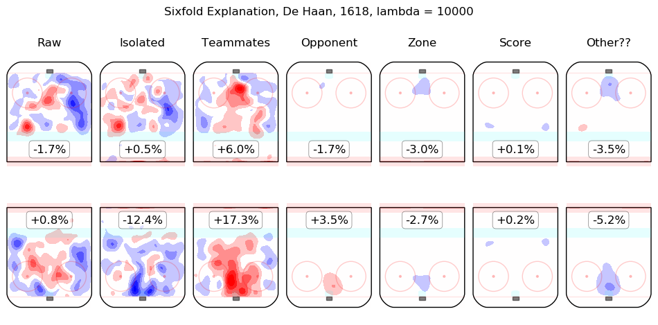
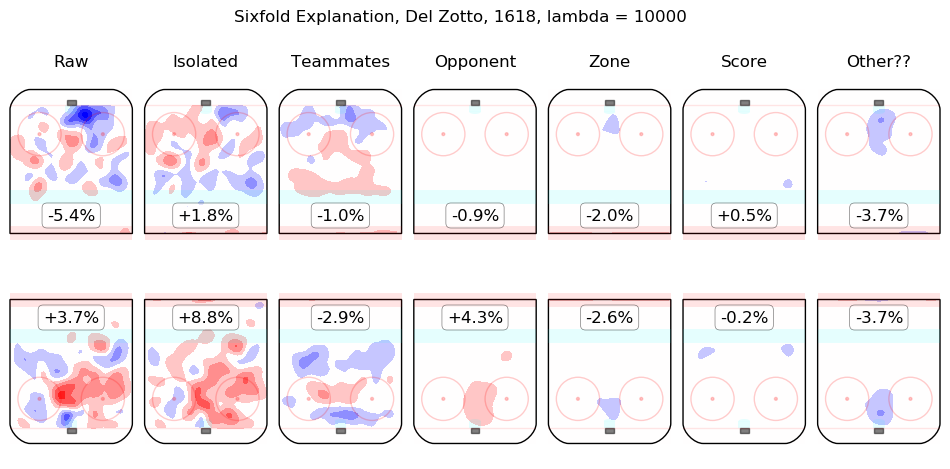
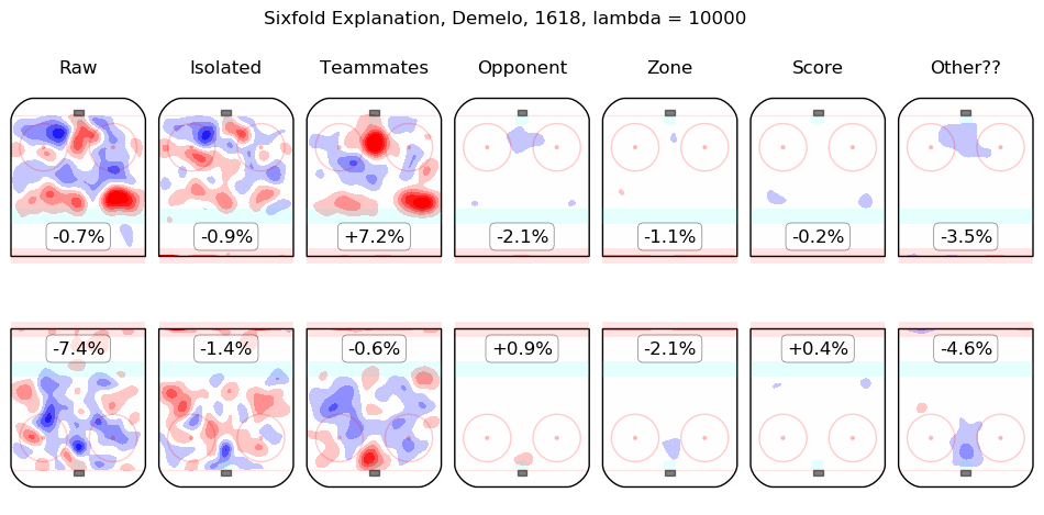
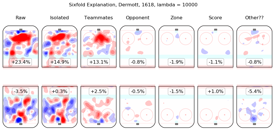
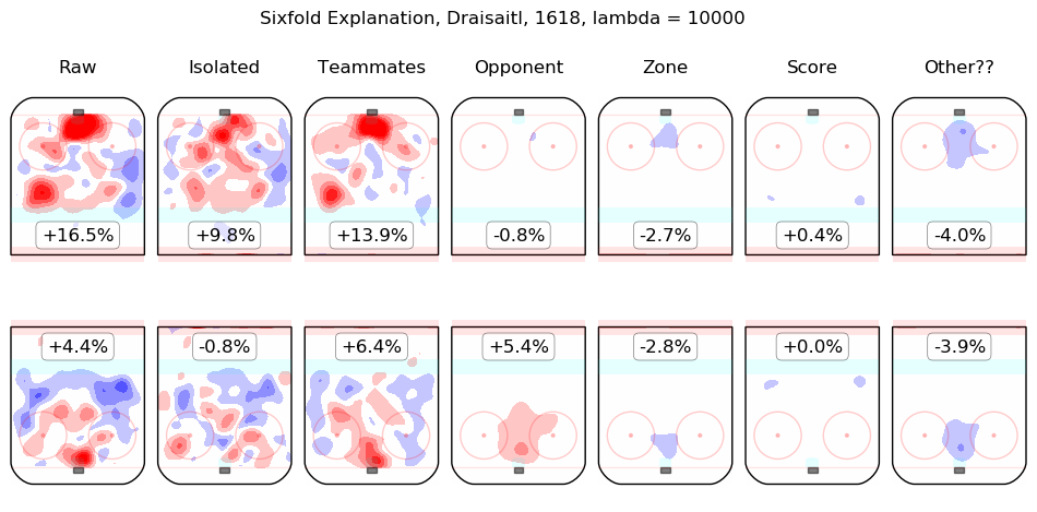
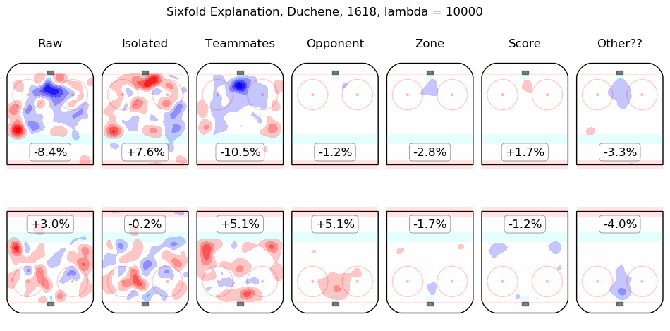
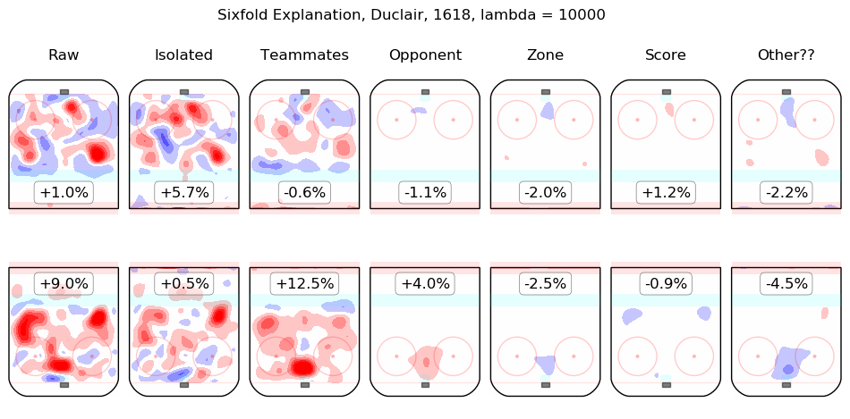
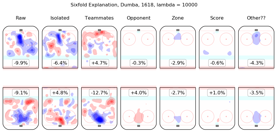
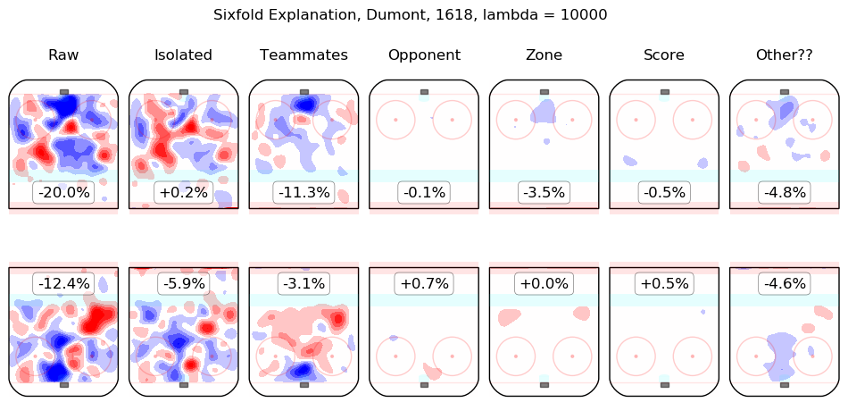
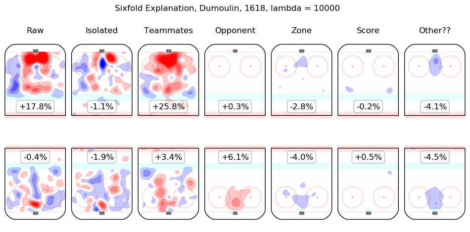
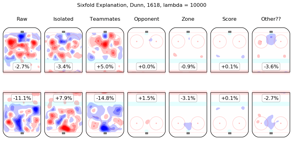
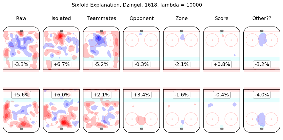
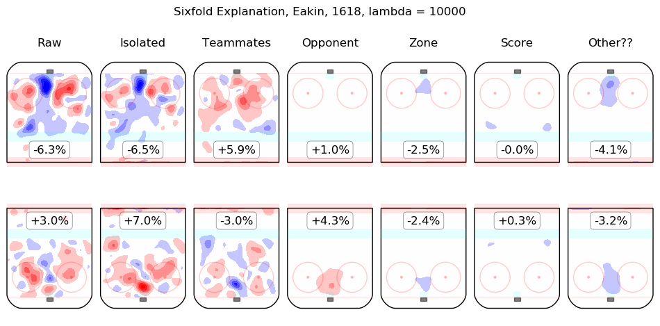
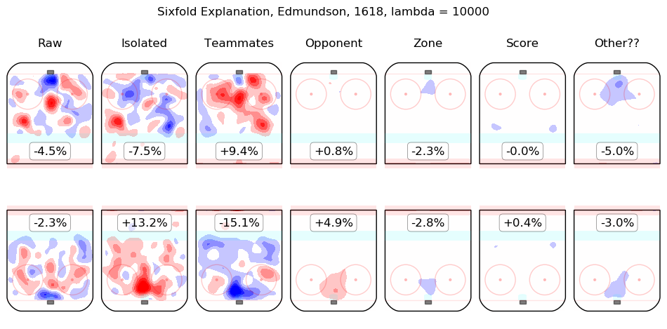
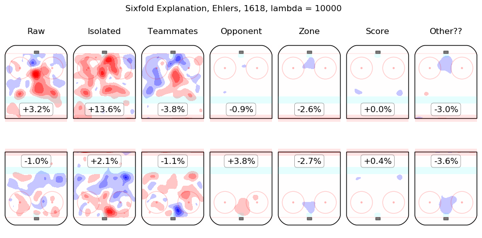
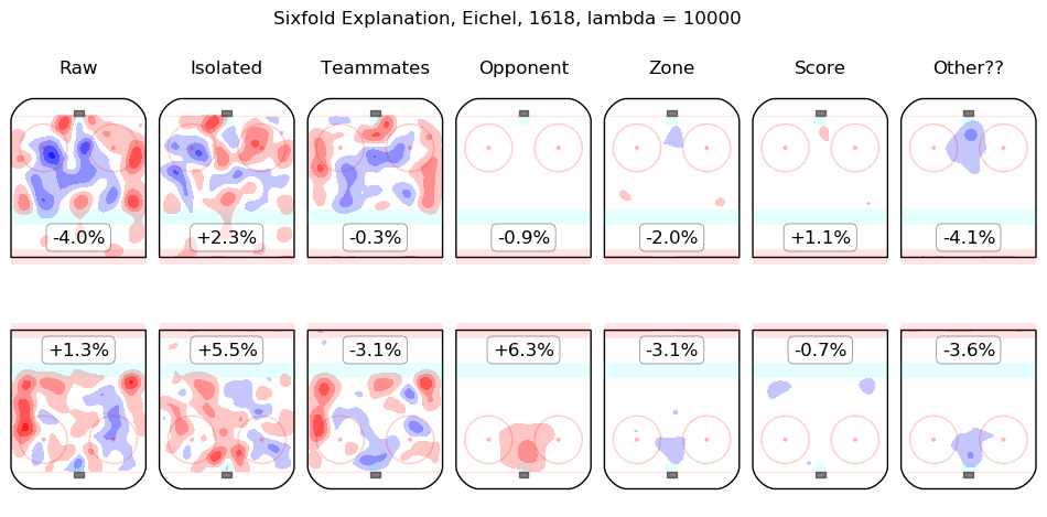
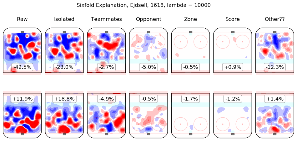
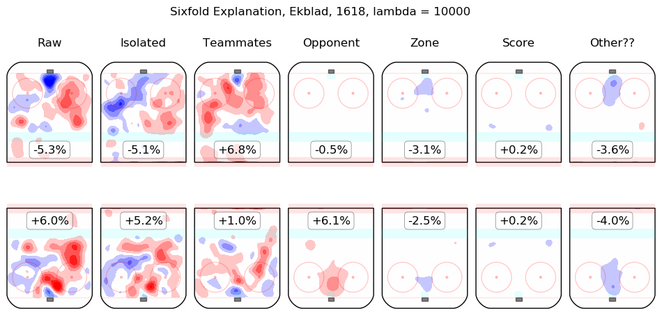
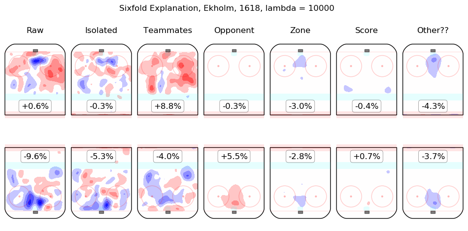
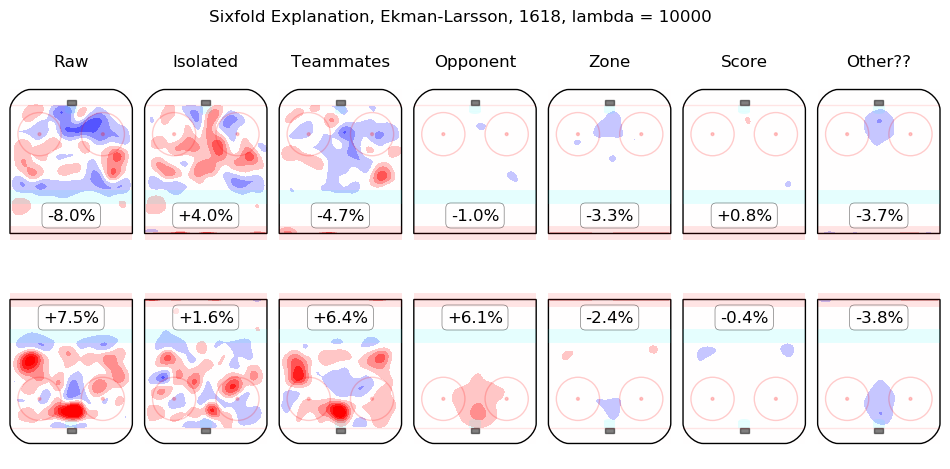
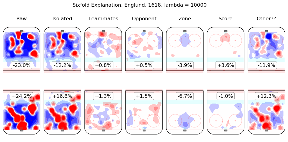
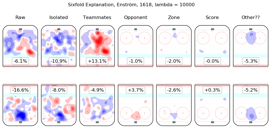
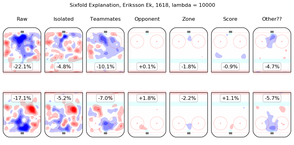
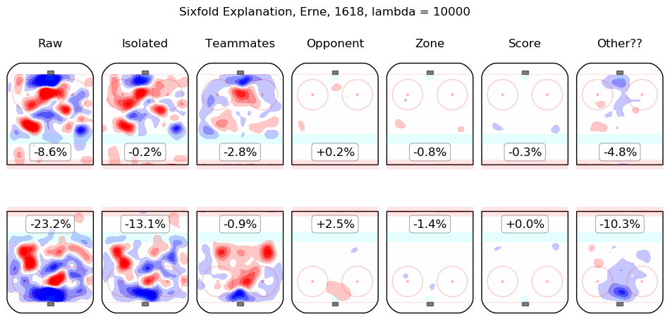
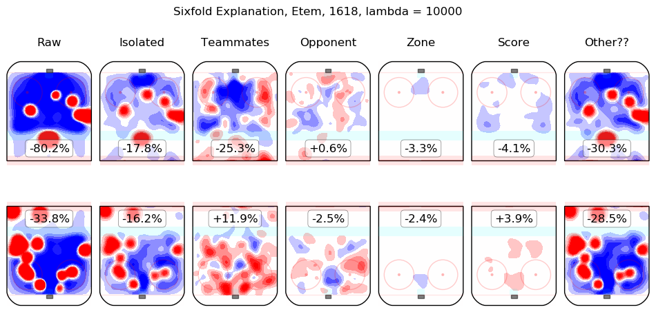
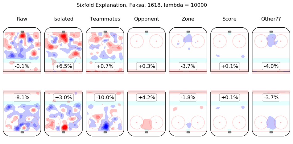
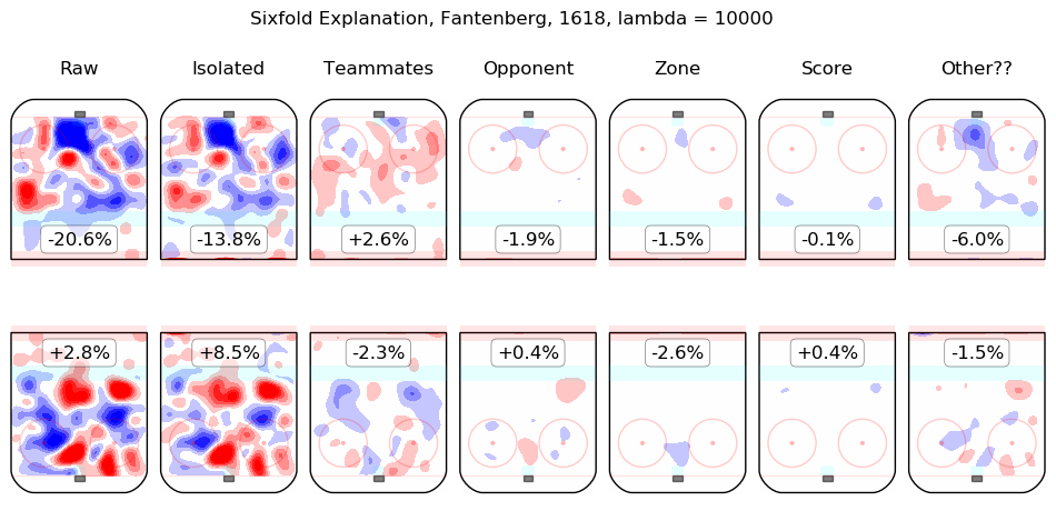
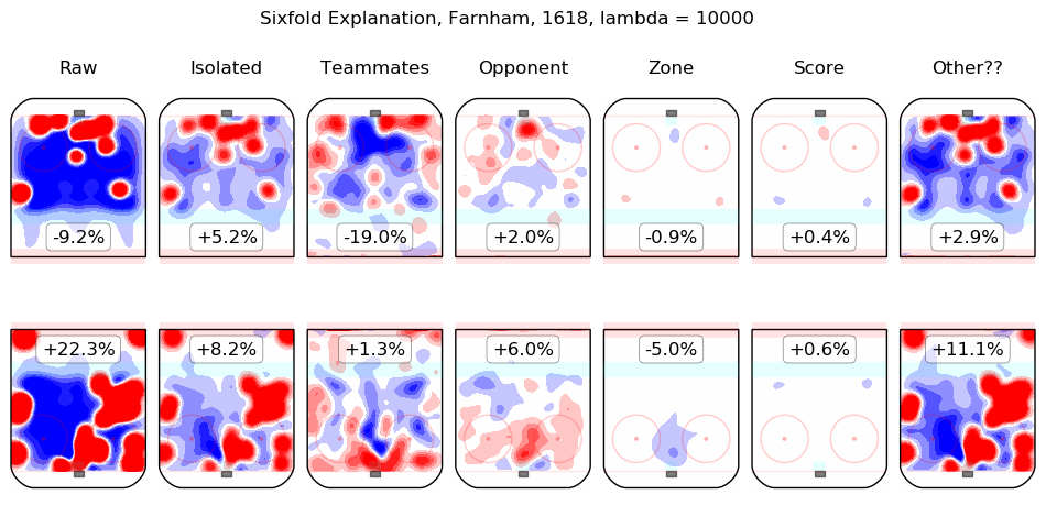
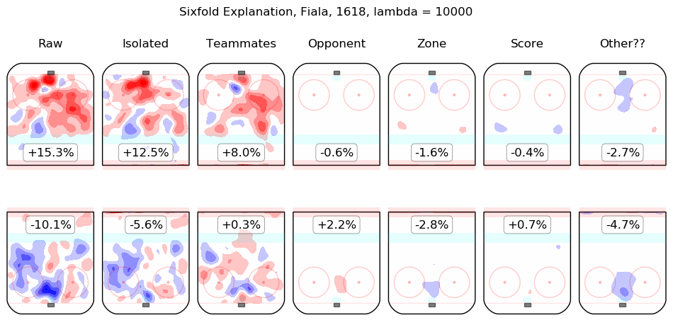
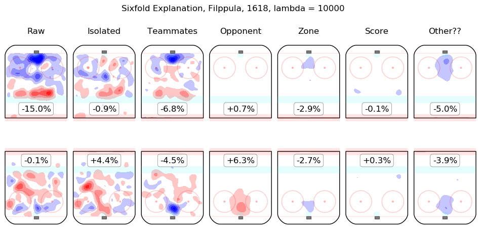
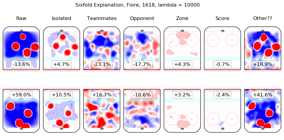
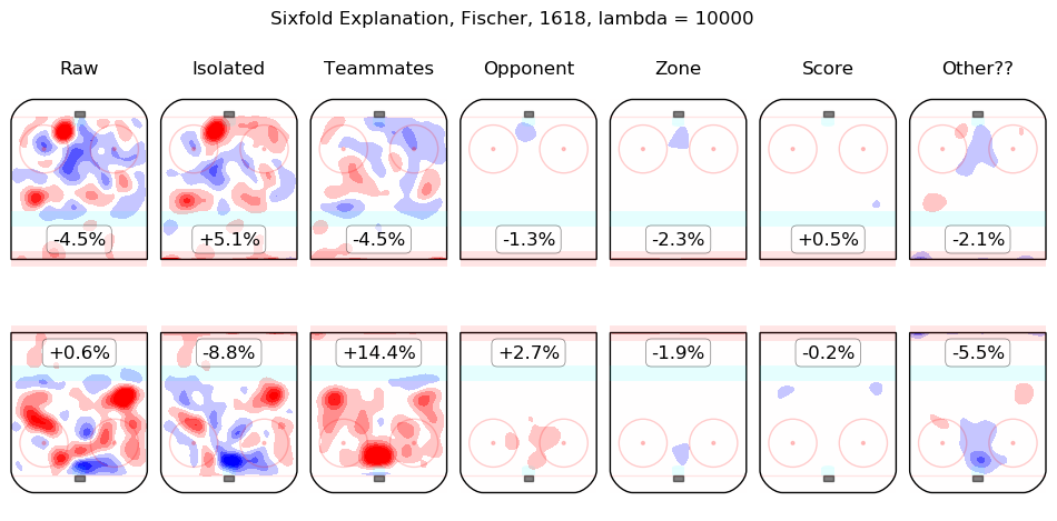
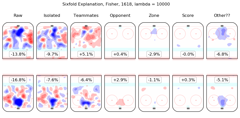
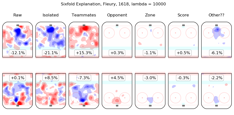
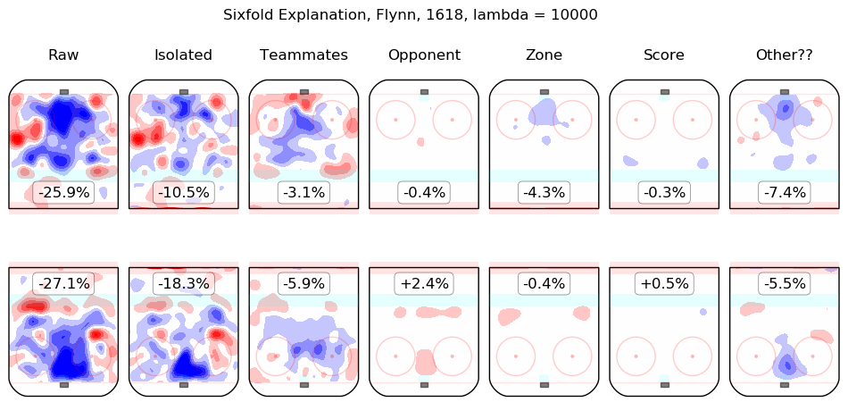
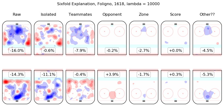
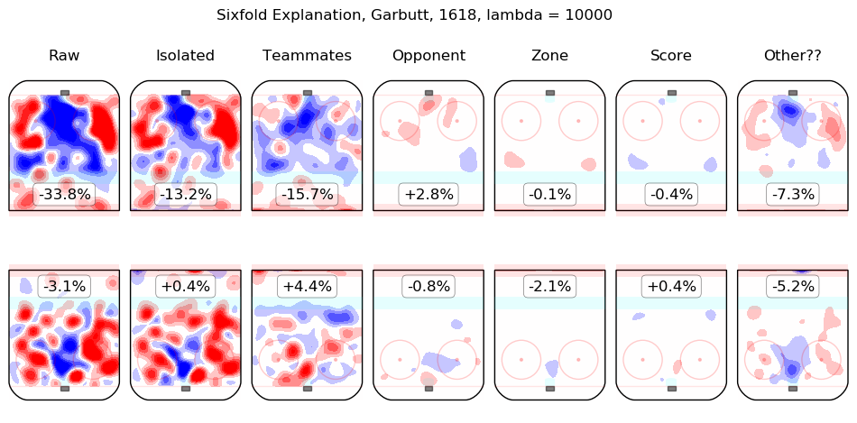
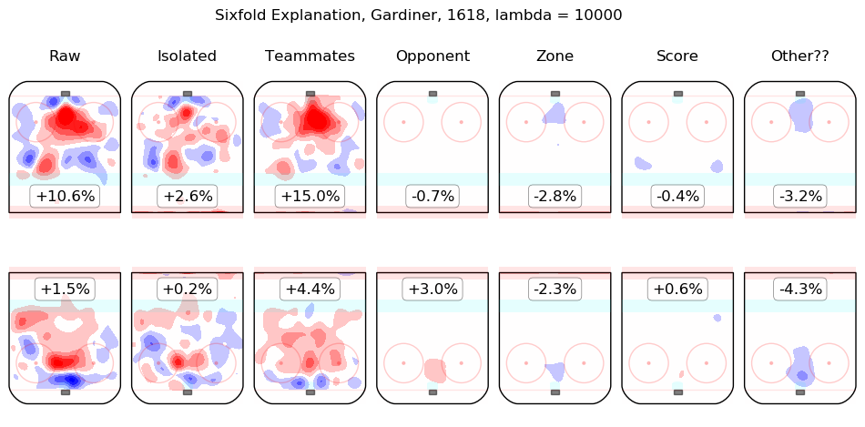
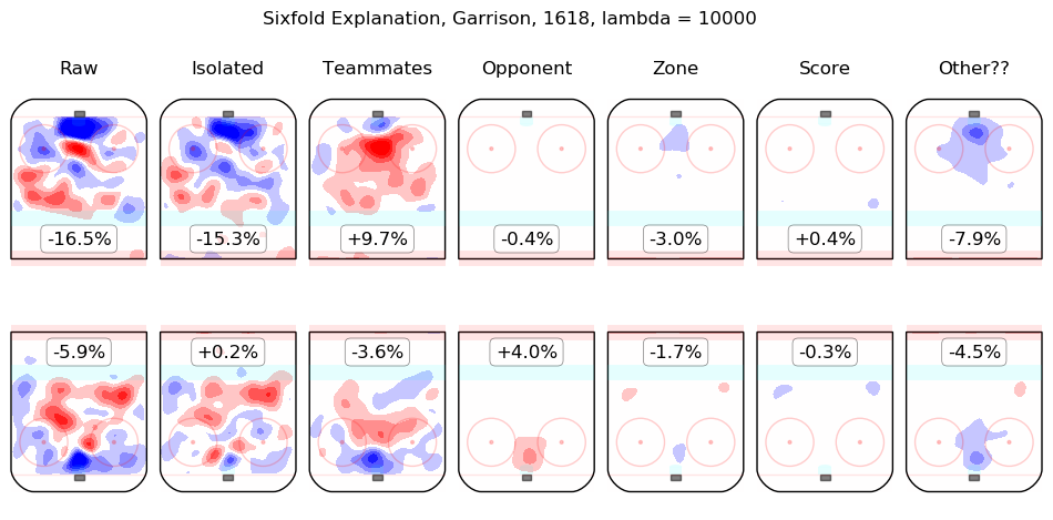
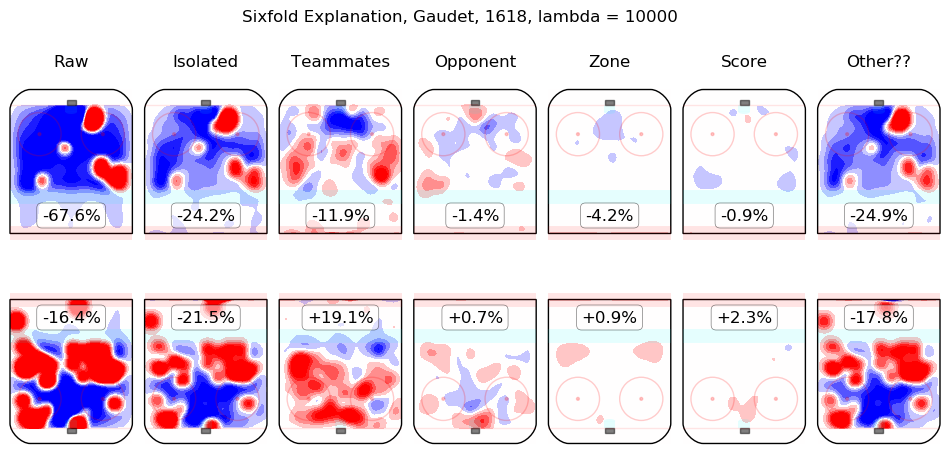
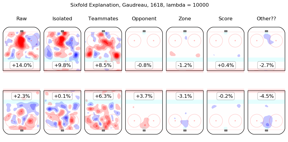
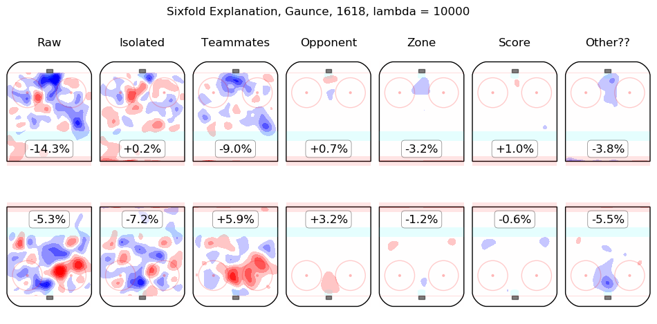
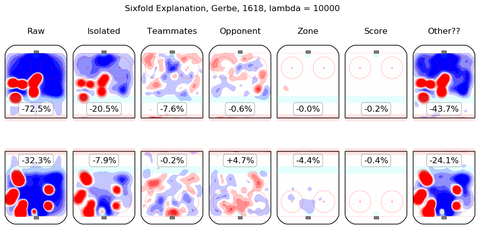
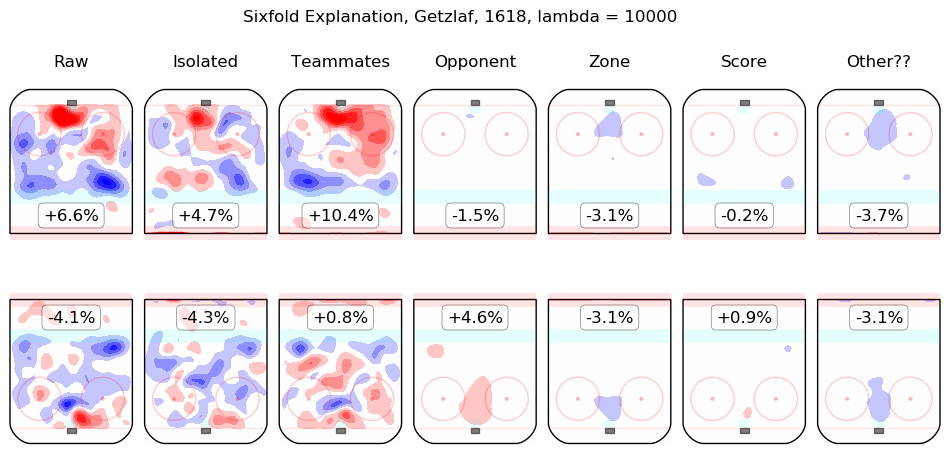
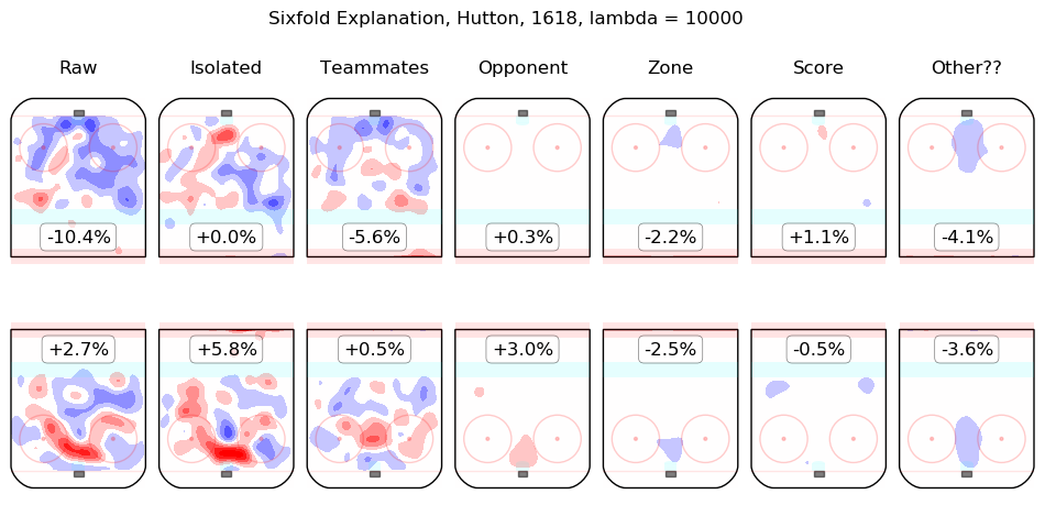
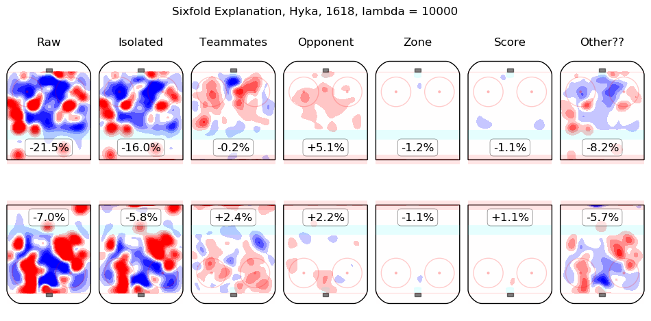
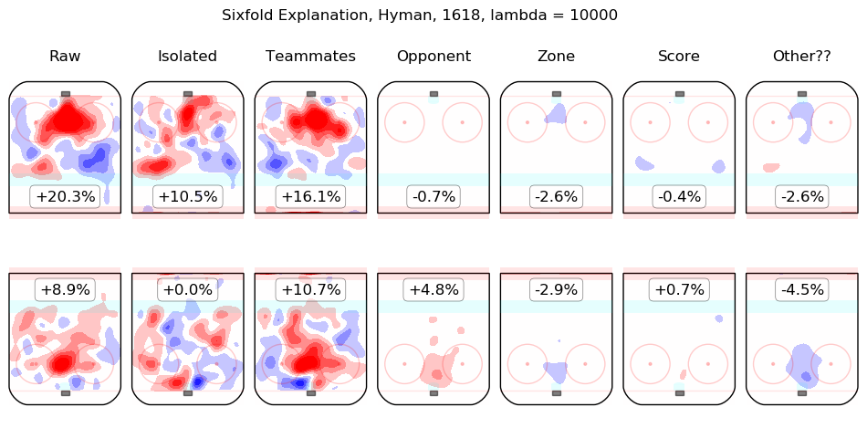
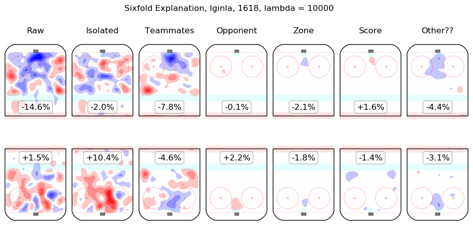
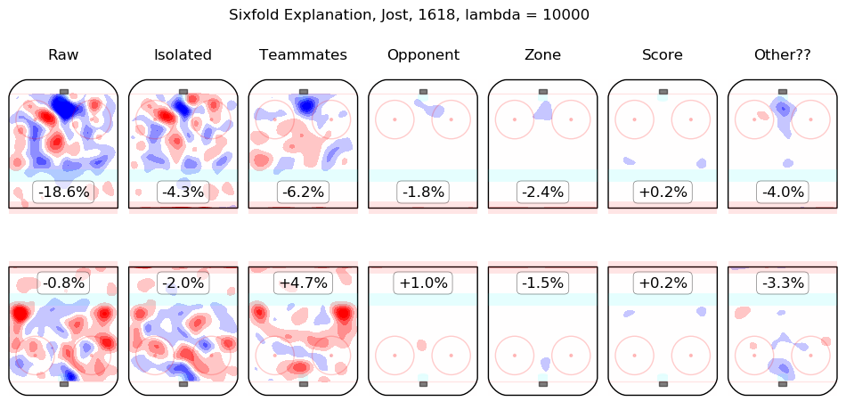
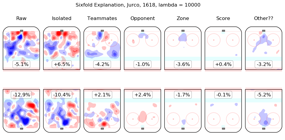
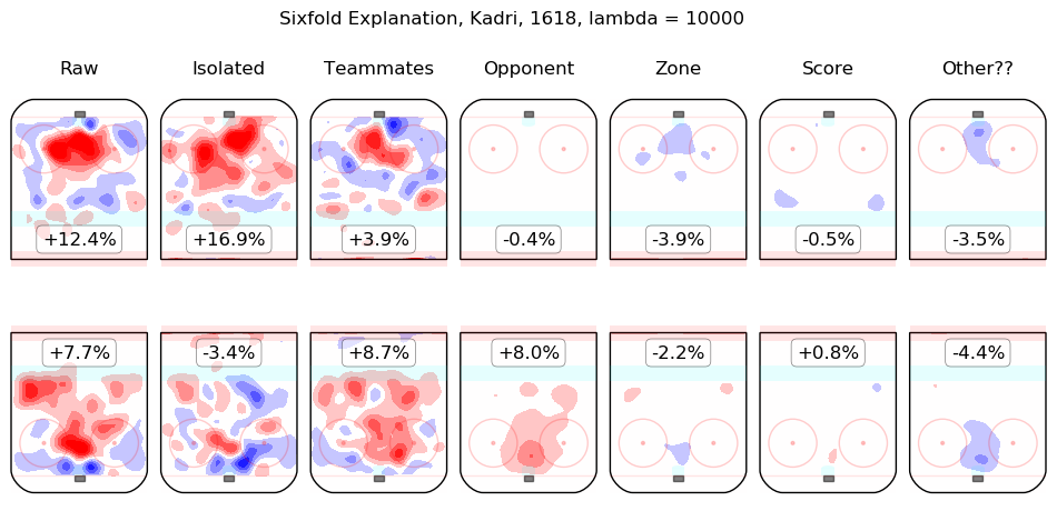
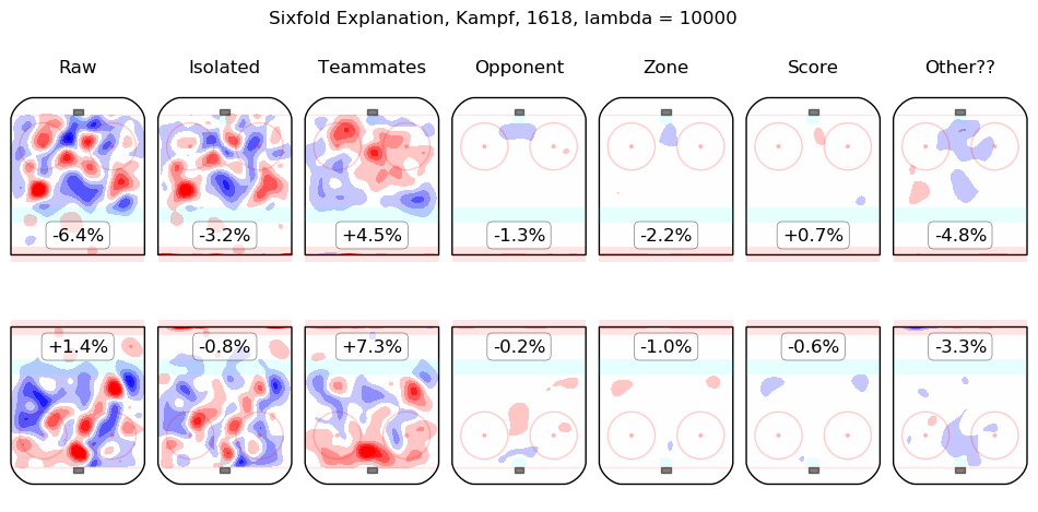
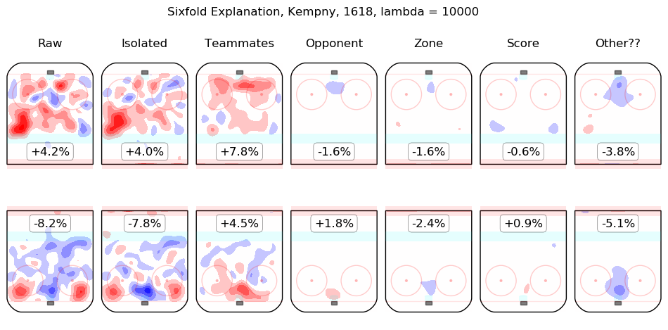
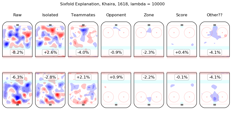
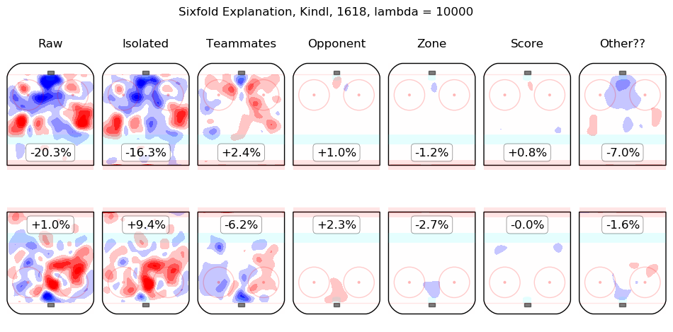
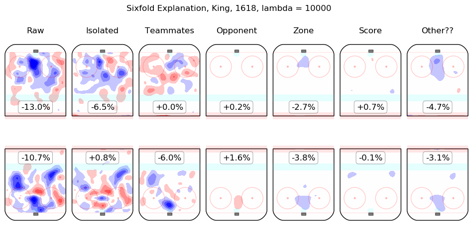
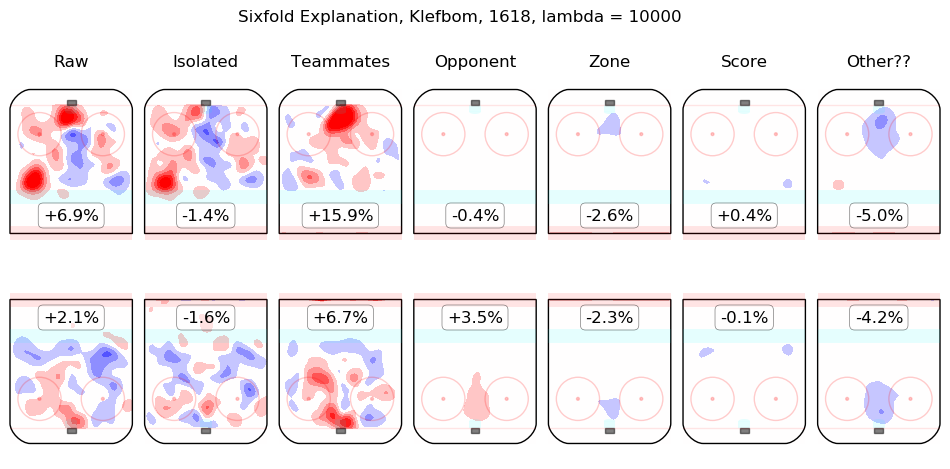
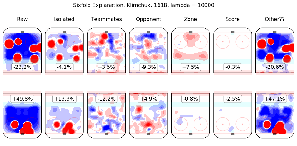
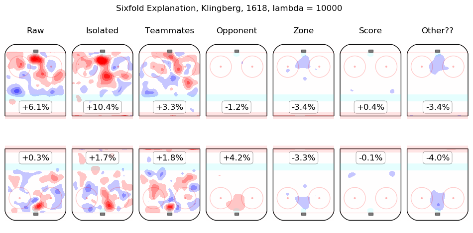
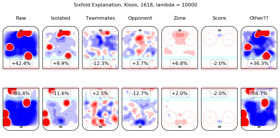
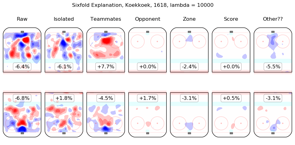
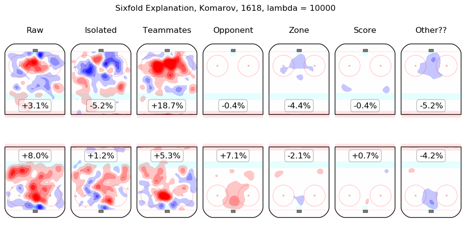
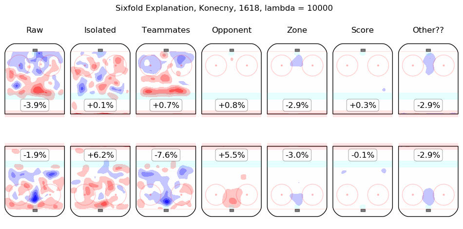
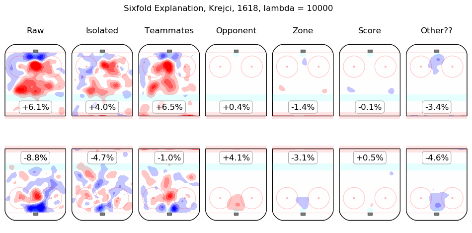
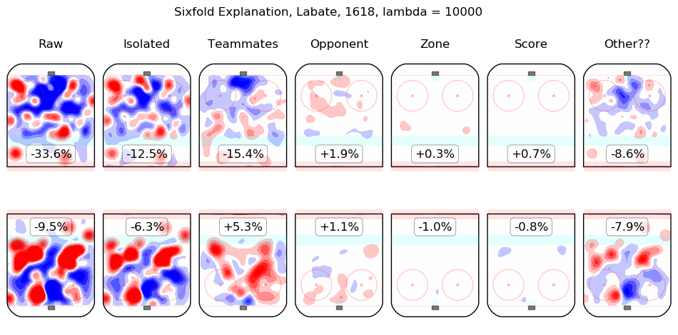
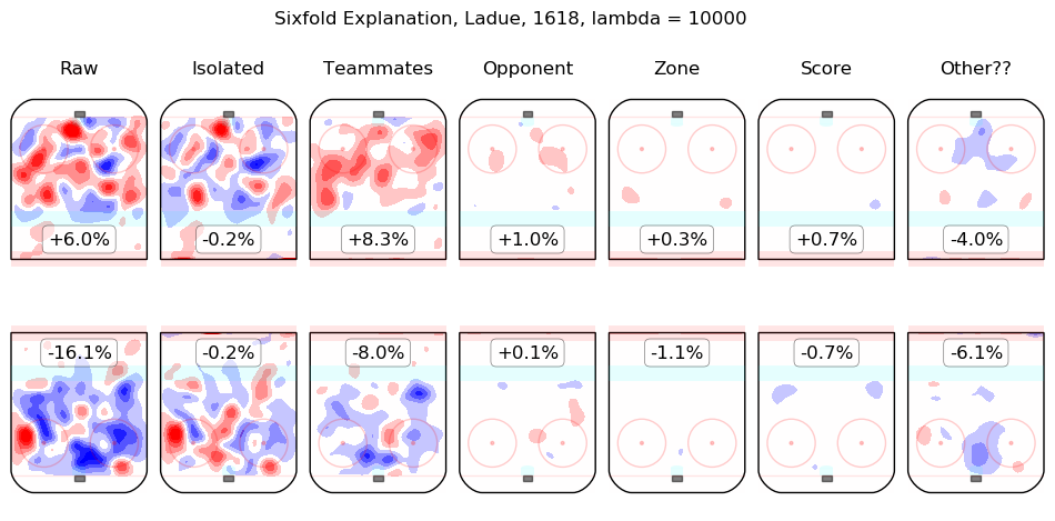
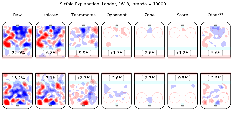
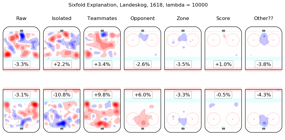
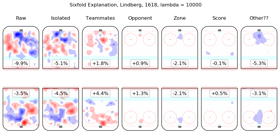
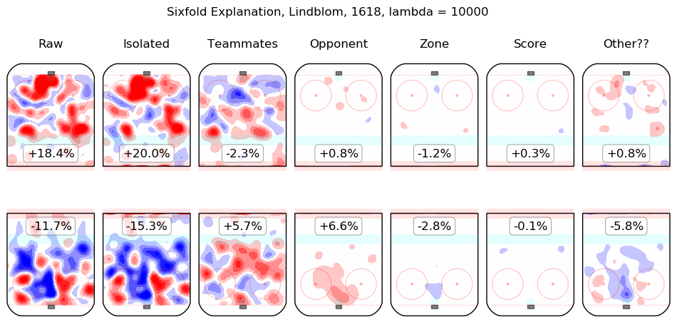
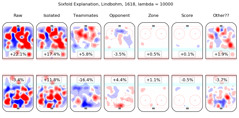
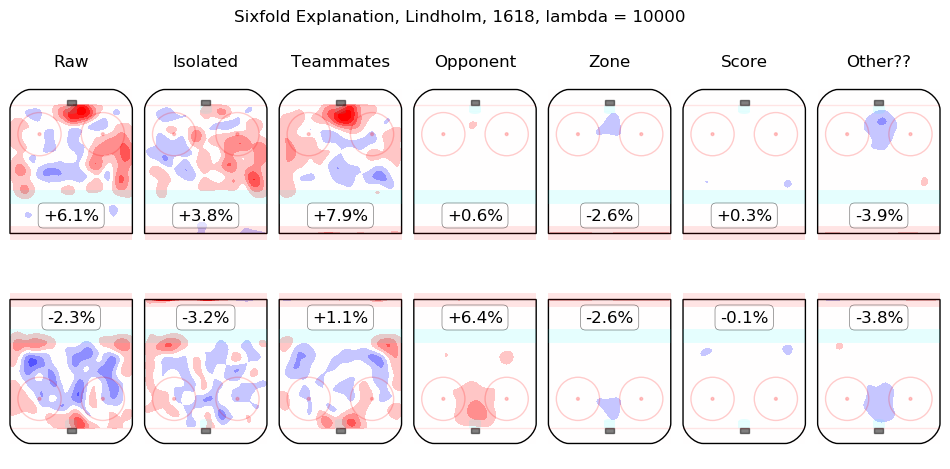
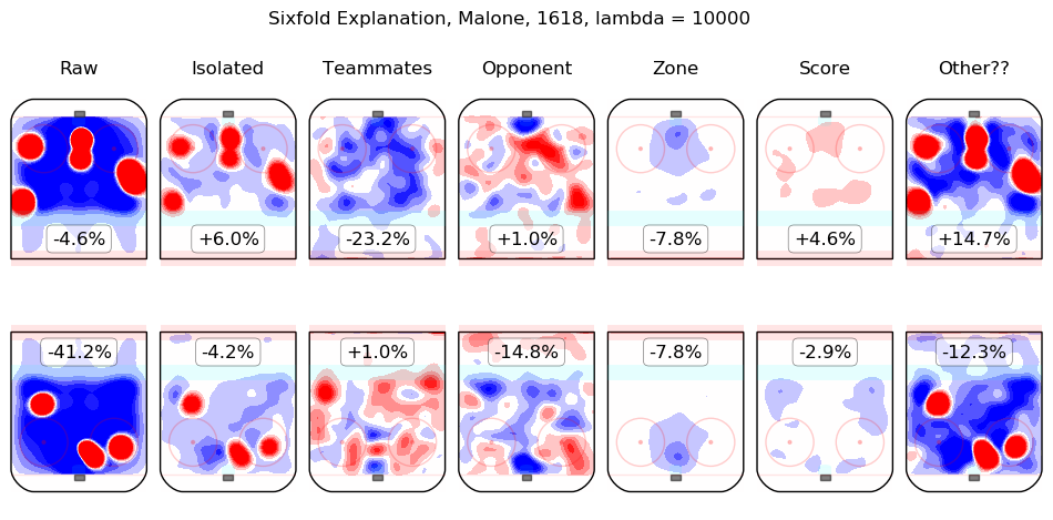
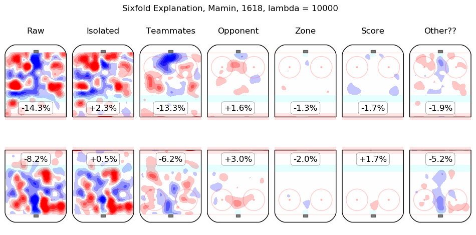
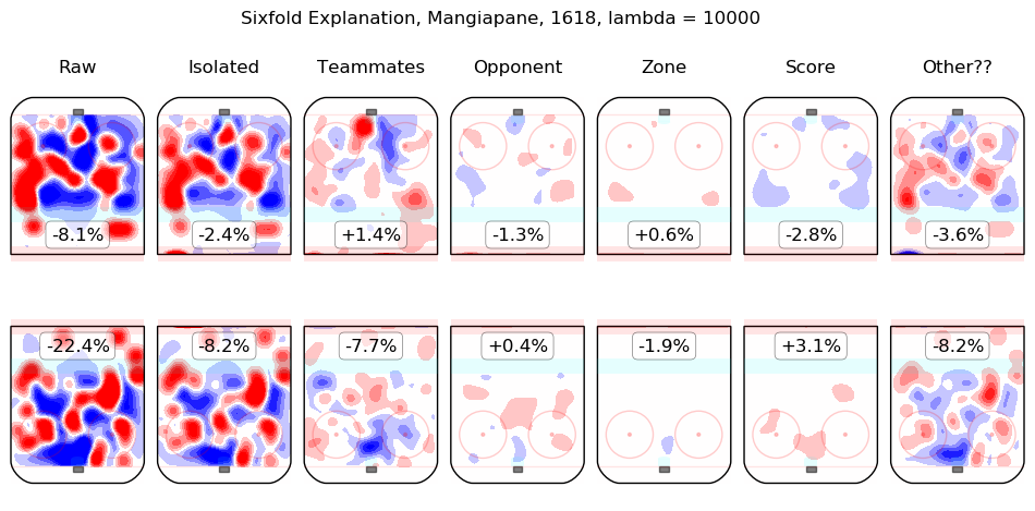
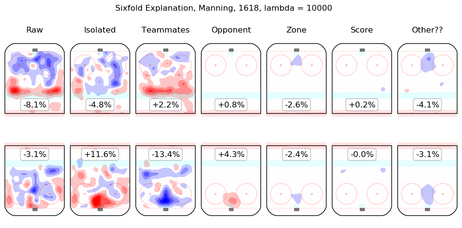
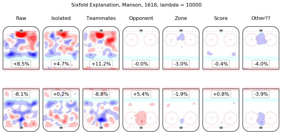
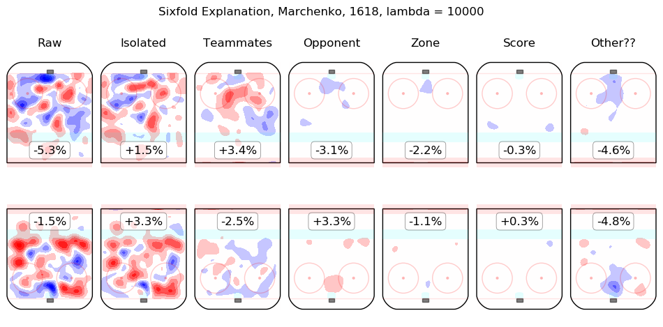
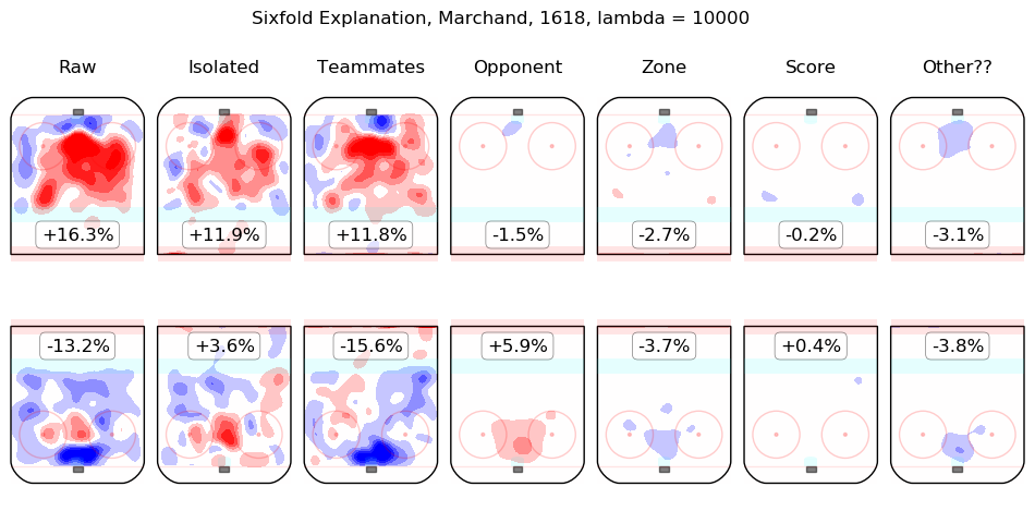
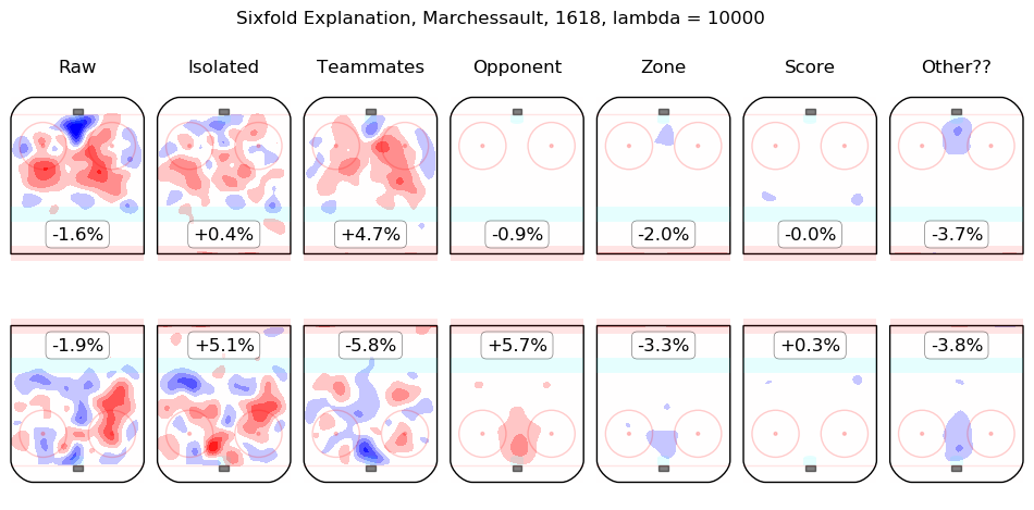
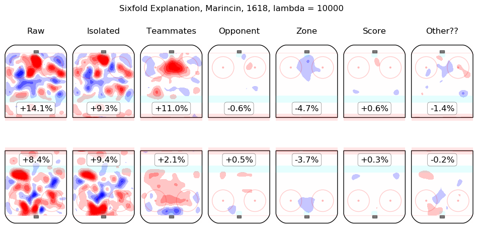
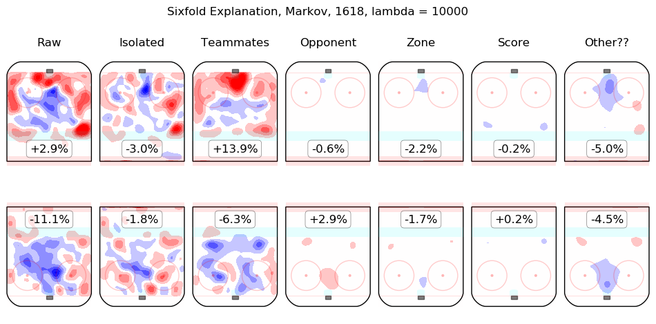
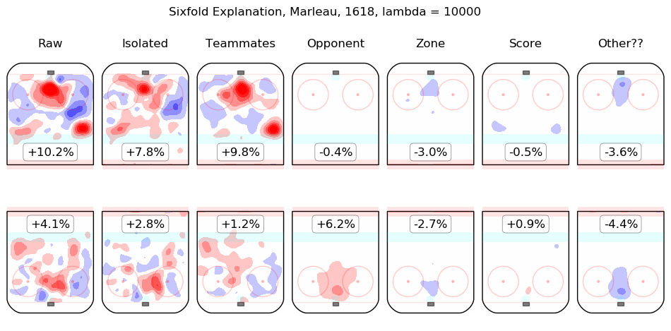
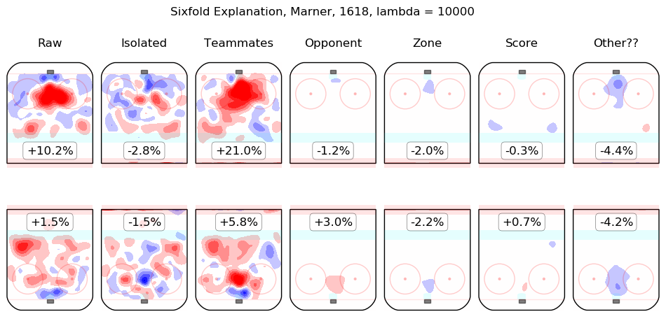
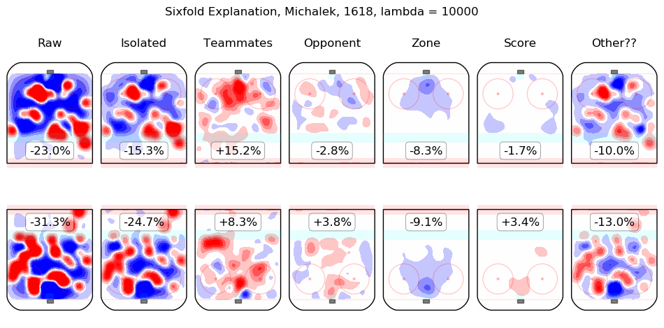
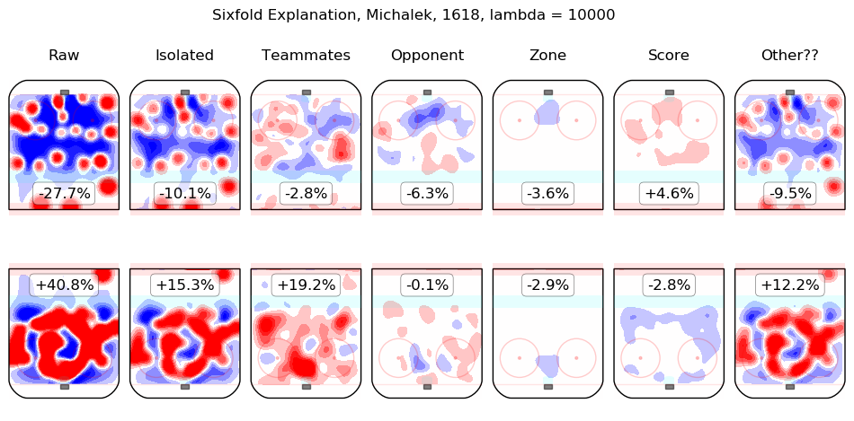
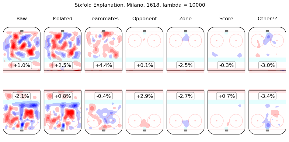
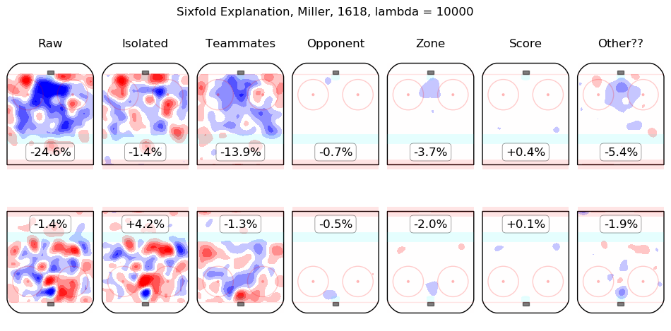
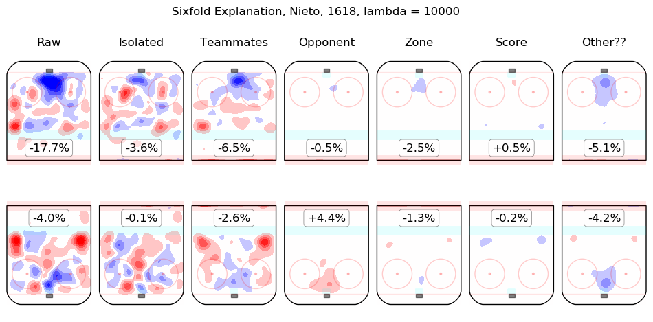
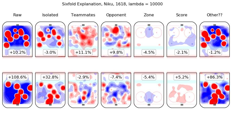
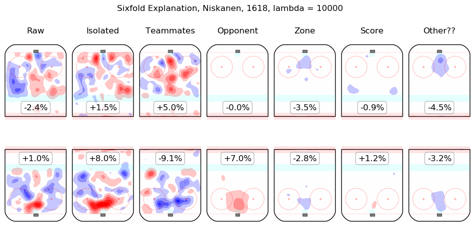
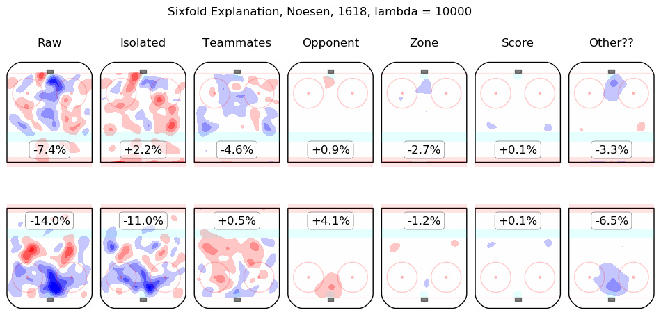
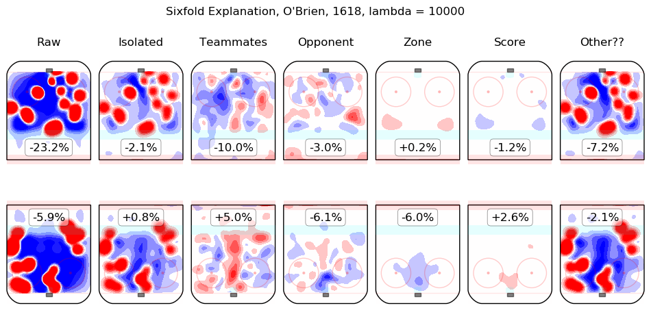
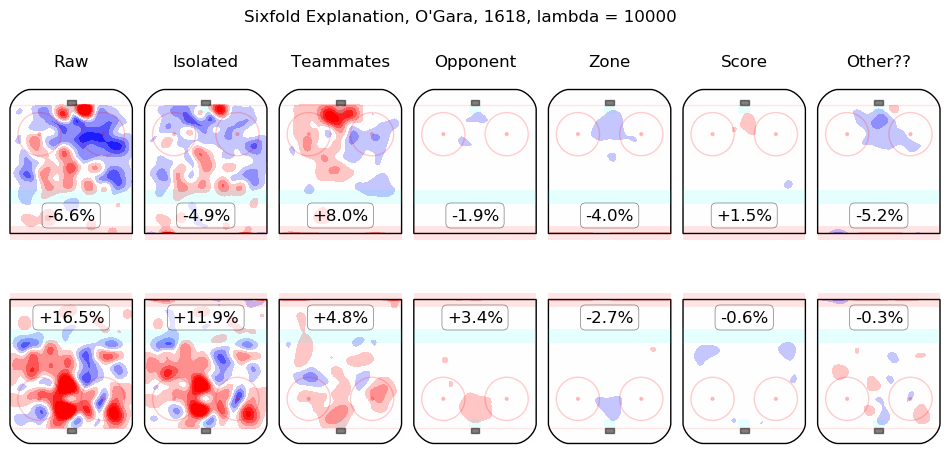
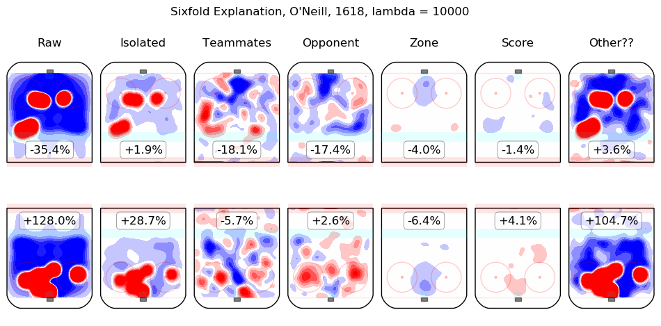
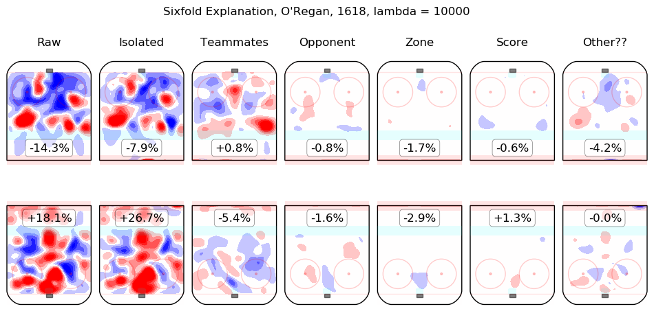
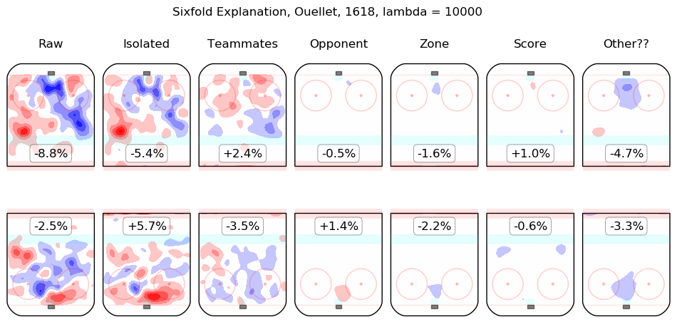
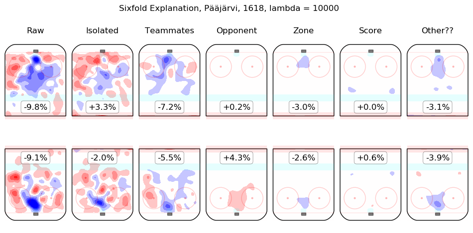
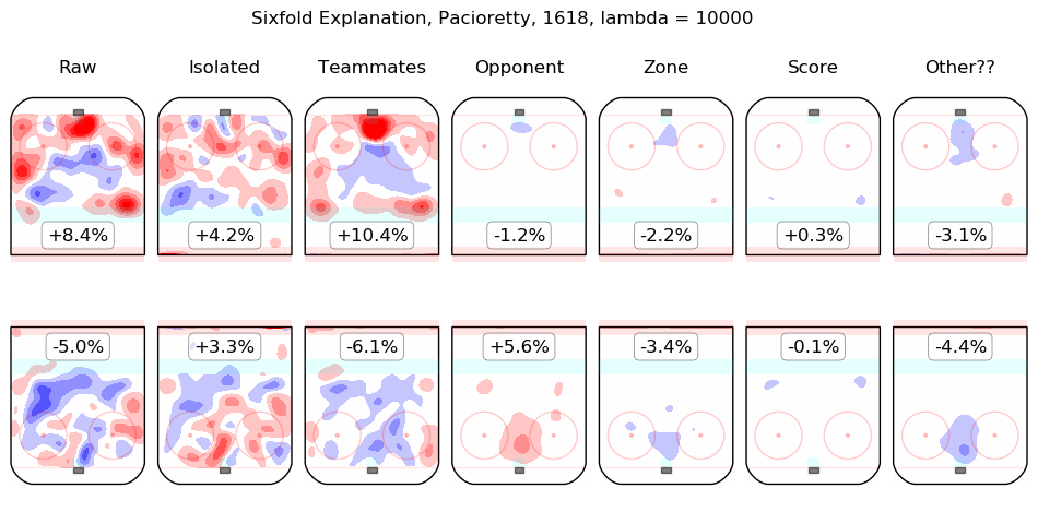
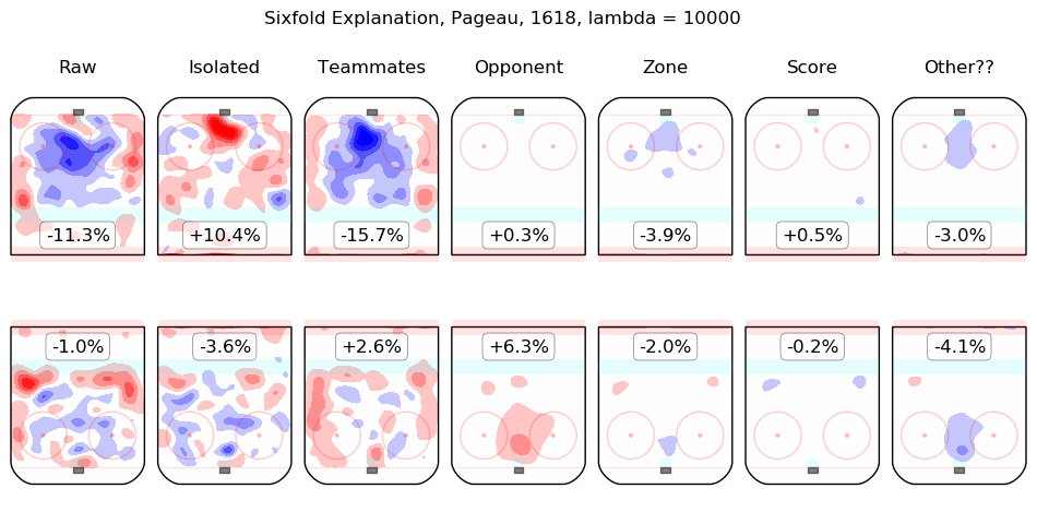
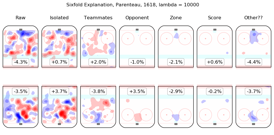
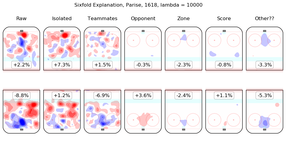
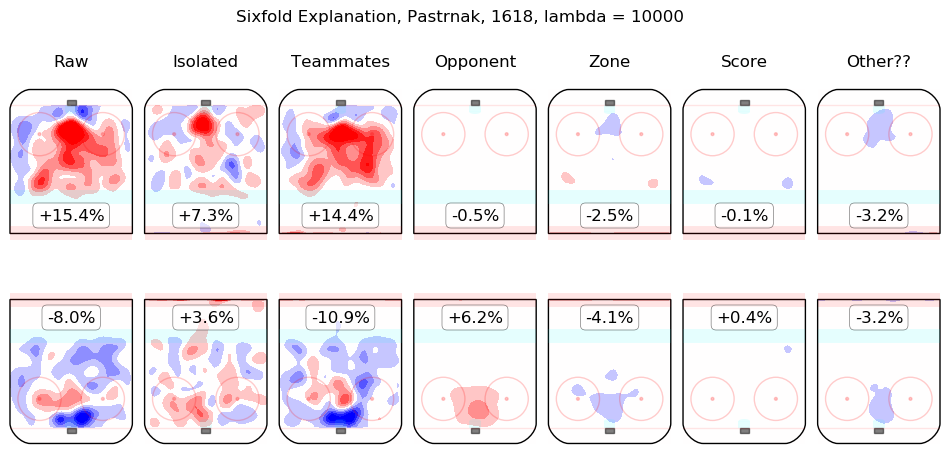
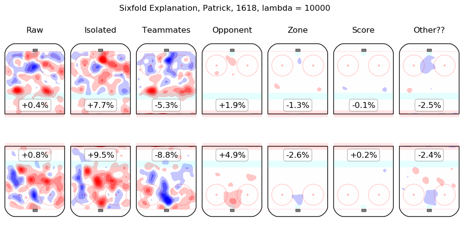
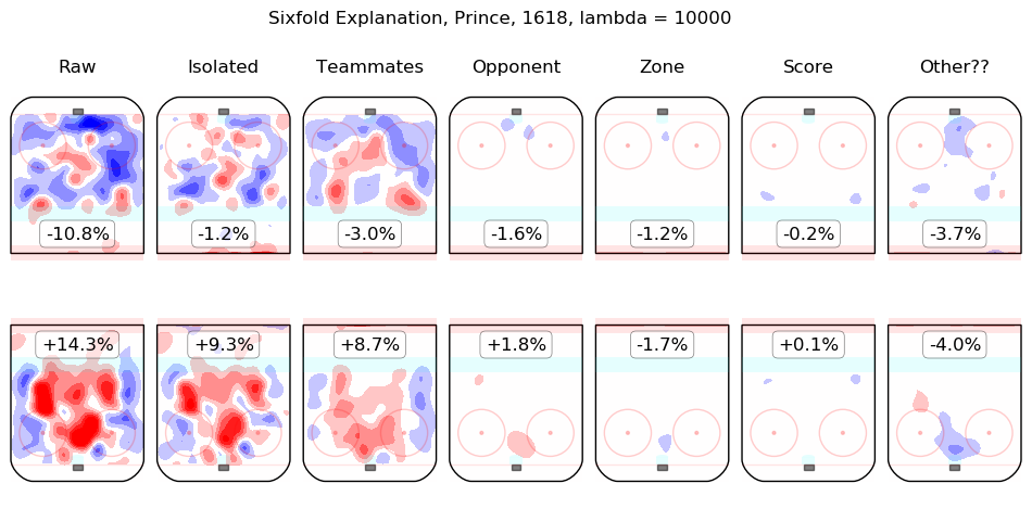
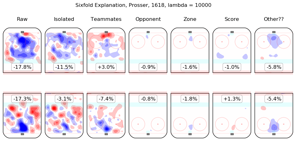
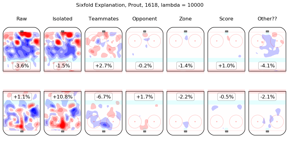
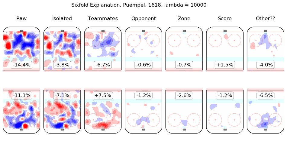
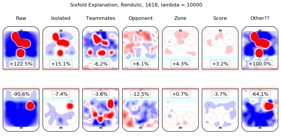
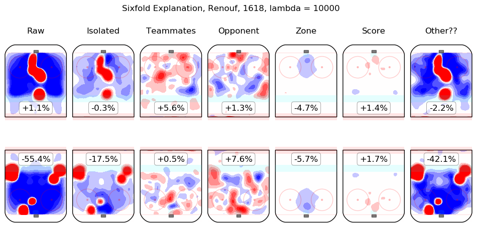
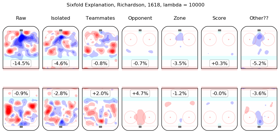
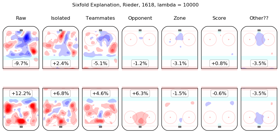
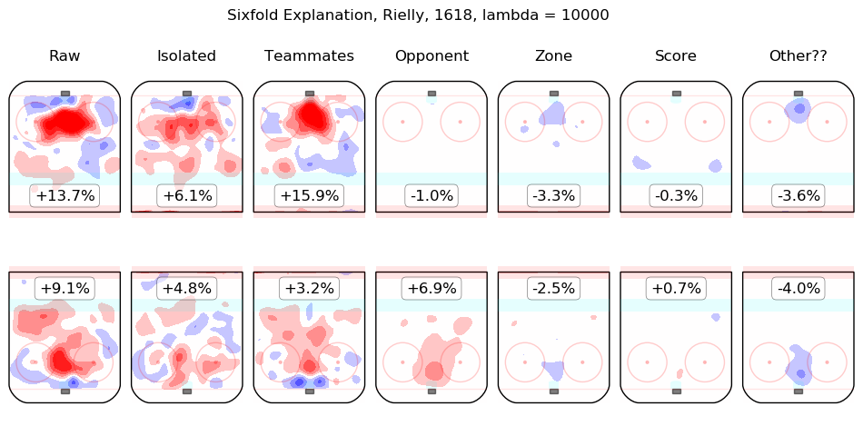
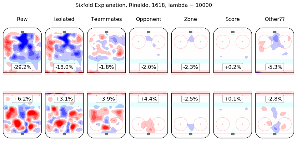
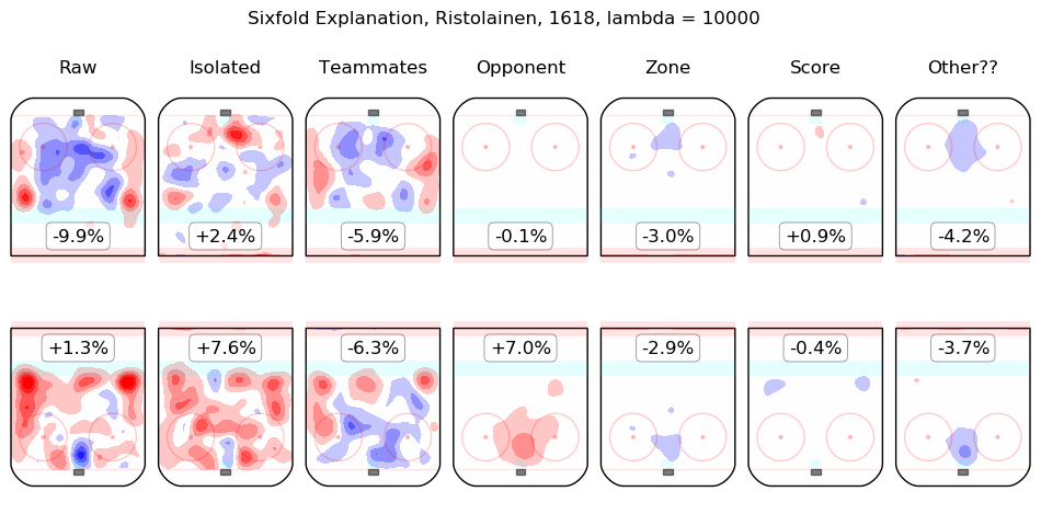
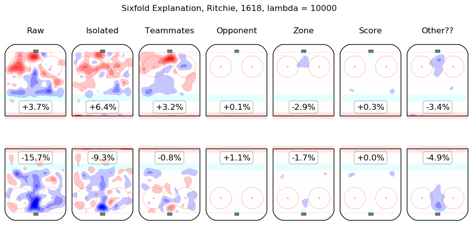
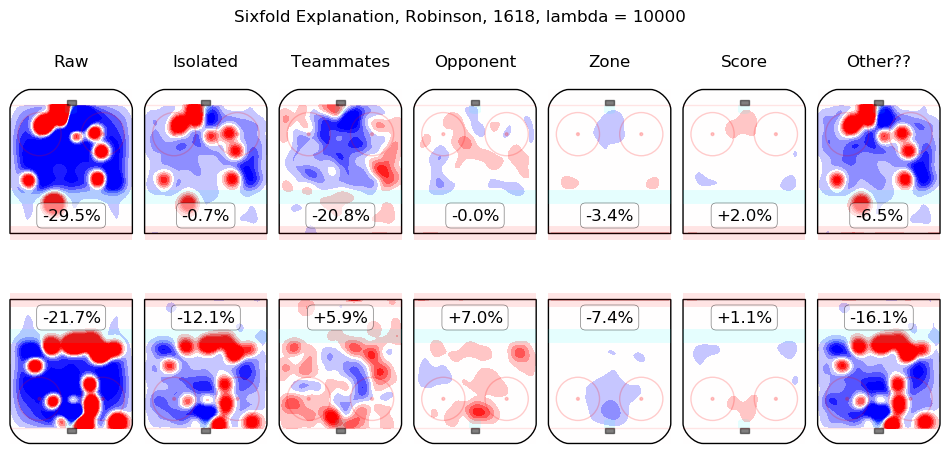
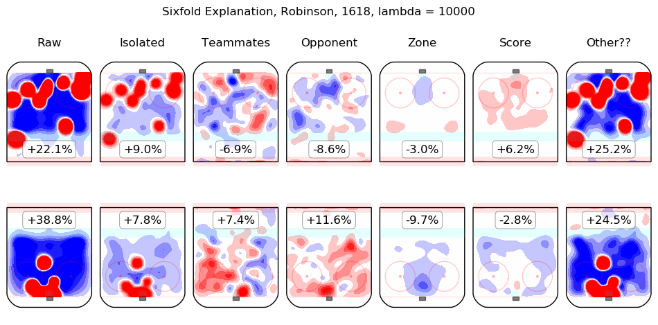
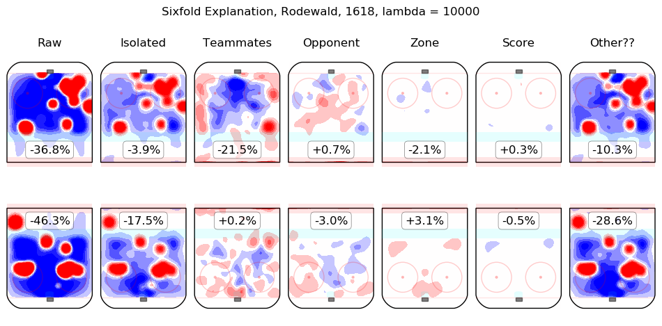
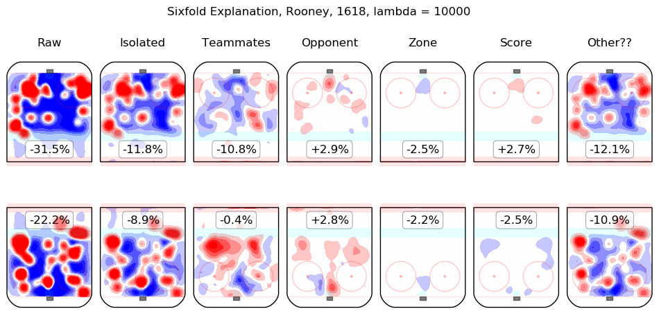
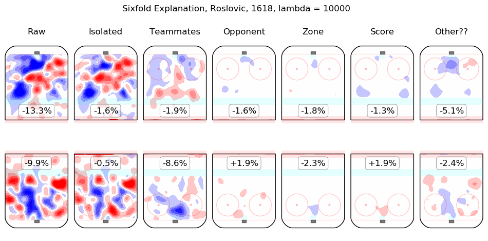
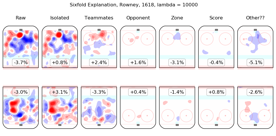
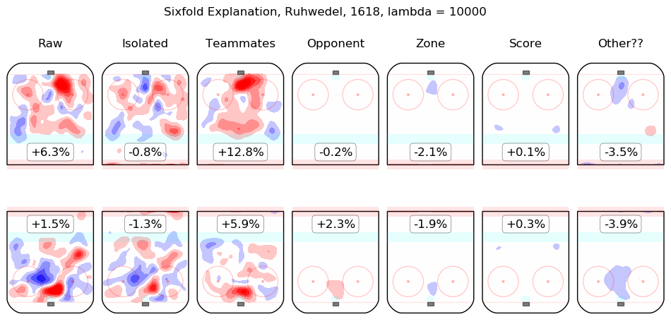
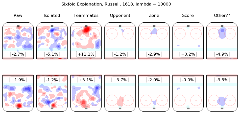
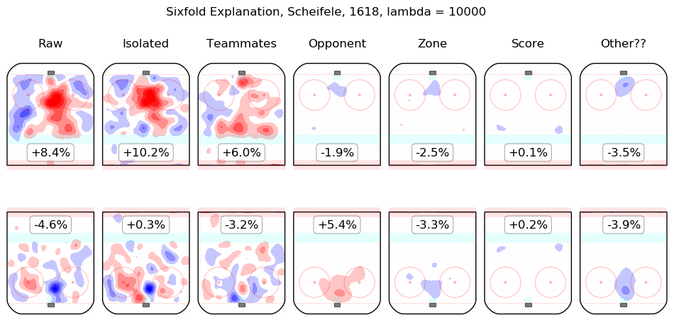
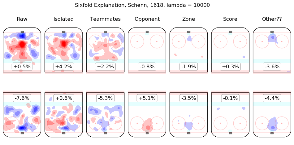
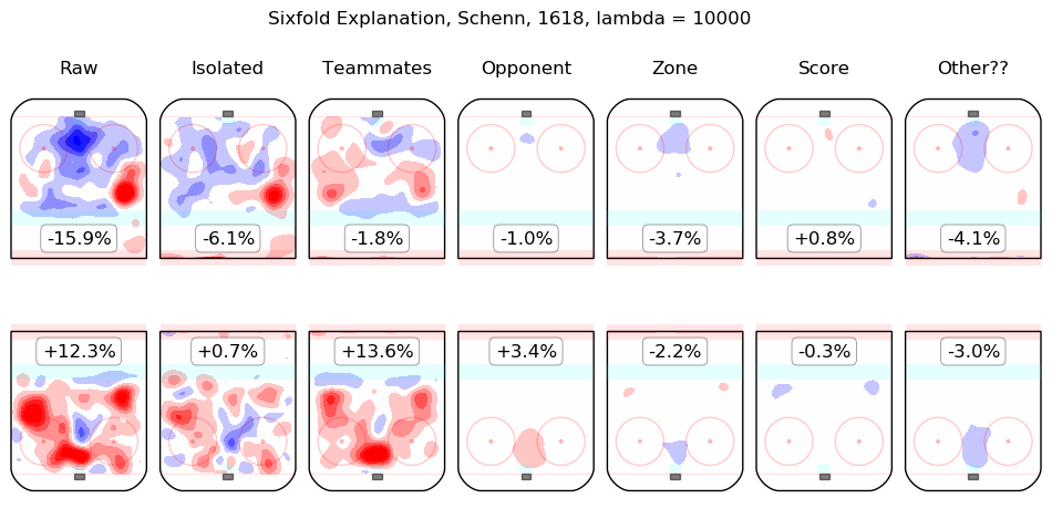
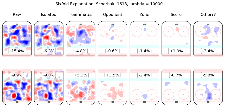
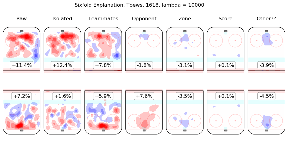
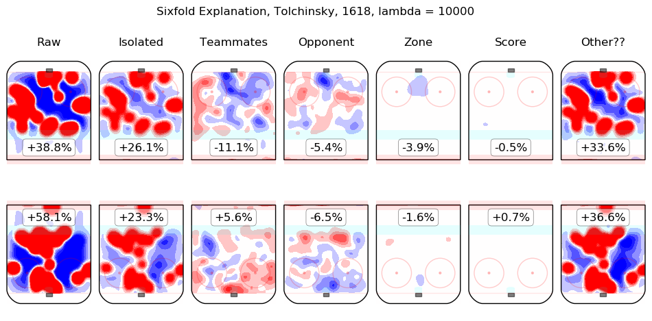
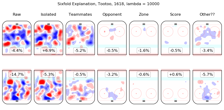
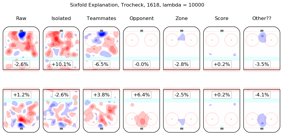
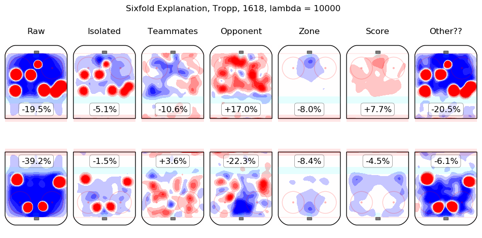
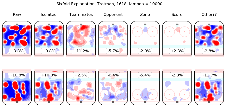
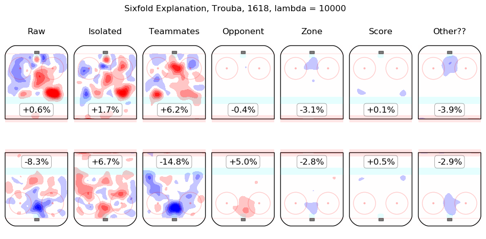
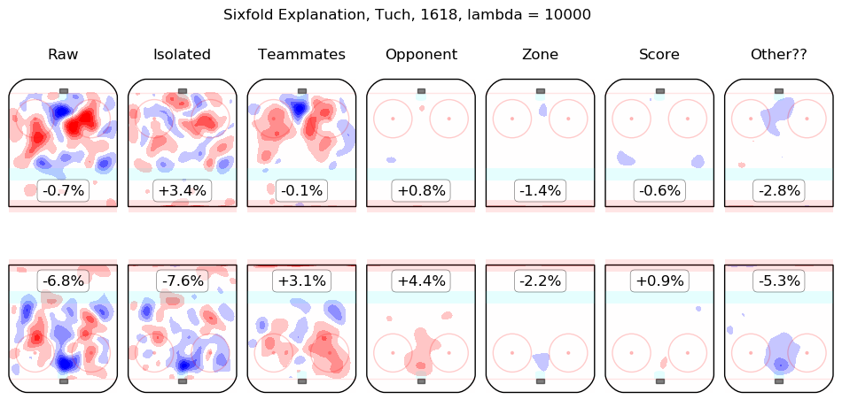
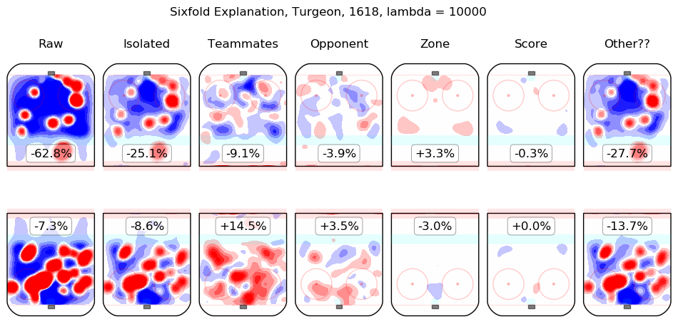
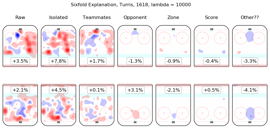
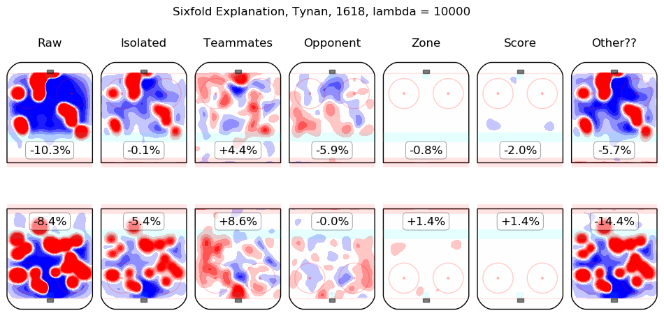
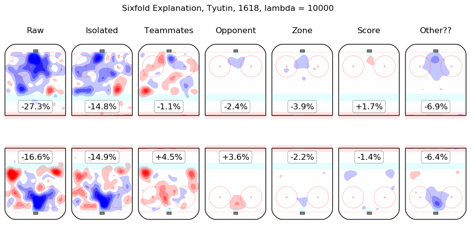
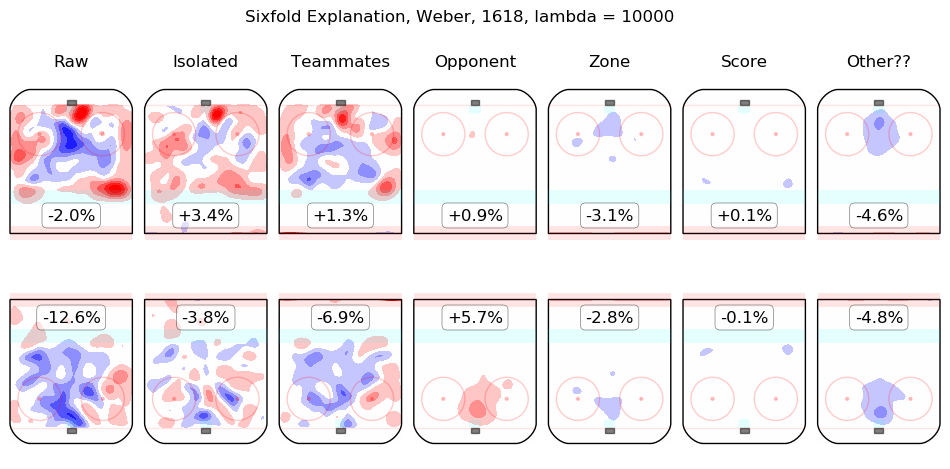
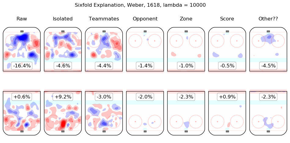
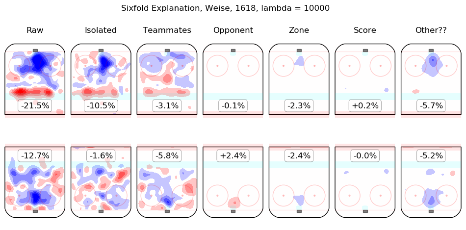
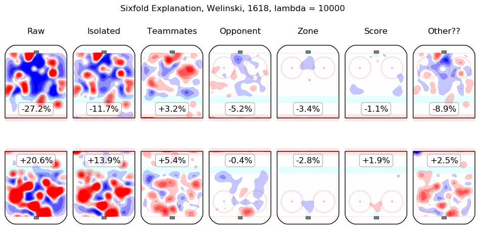
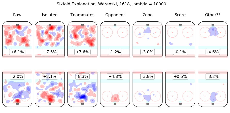
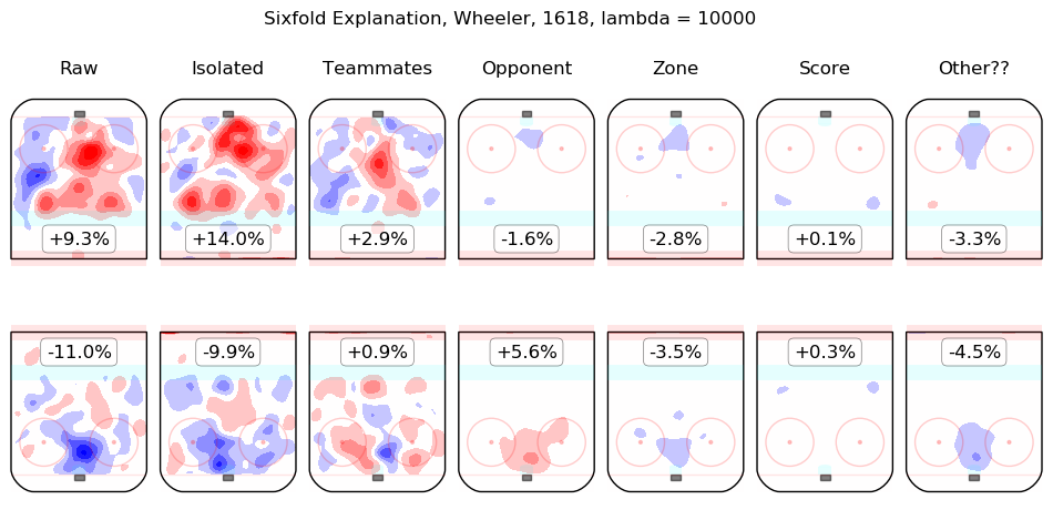
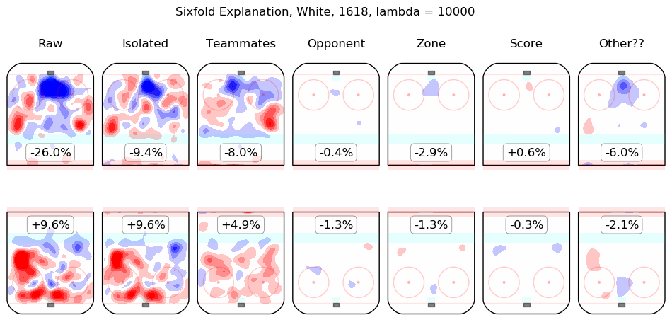
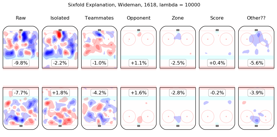
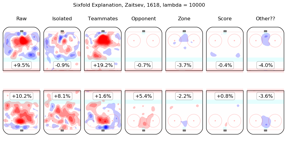
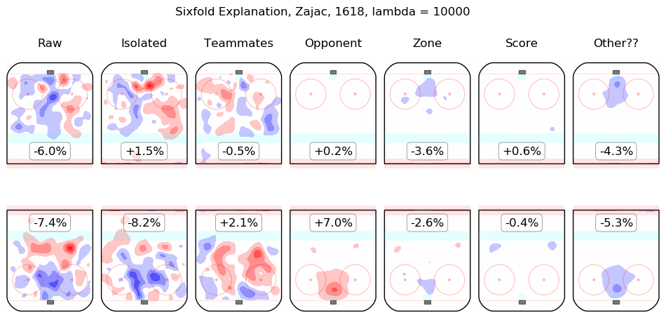
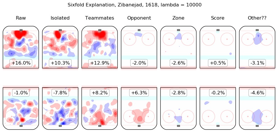
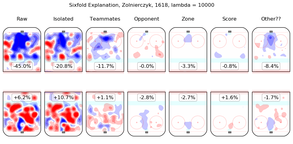
In time I will integrate measurements from this model throughout the site. For the moment, I content myself with the following list of summary graphics for all 2016-2018 skaters. To illustrate how they are to be read, consider the summary graphic for Taylor Hall, below:
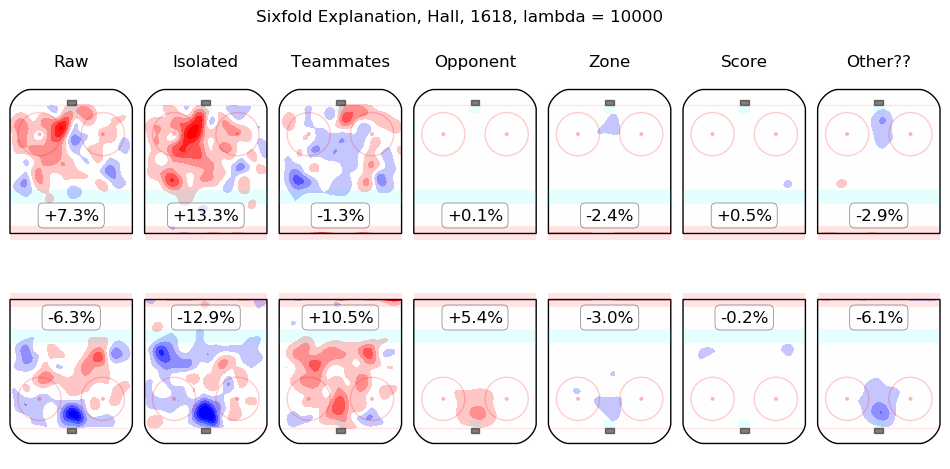
The first column shows the on-ice observations from Hall's 5v5 minutes with New Jersey in the 2016-2017 and 2017-2018 regular seasons. Even considering only shot rates, they were good, from his point of view, with his team generating offence 7.3% more threatening than league average while his opponents generated 6.3% less threatening offence than league average. The "isolated" column is the pair of regression outputs for Hall himself; his individual impact is to create a great deal of offensive threat (+13.3%) and also to strongly suppress shots against (-12.9%). His teammates, in weighted sum, are shown in the "teammates" column, they are responsible for a slight drop in offence (-1.3%) and a hefty increase in shots against, +10.5%. The impact of his opponents is shown in the "opponent" column; his opponents do not particularly affect the shots the devils are expected to generate (+0.1%) but are strong offensively themselves and are thus expected to contribute +5.4% offensive threat to New Jersey's opponents. The zone impacts are slightly negative for both offence and defence, the score impacts are negligible in aggregate (as one might expect for a close-to-average team like New Jersey, who spend a lot of time in every score state). Finally, the "Other??" column is the "residuals" described above and are both negative, which is to say, the raw results for both offence and defence when Hall was on the ice are both lower than the model estimates for all of the relevant features. In sum, Hall is, as most observers have suggested, personally driving the play, both offensively and defensively, in the teeth of weak teammates and tough opponents.
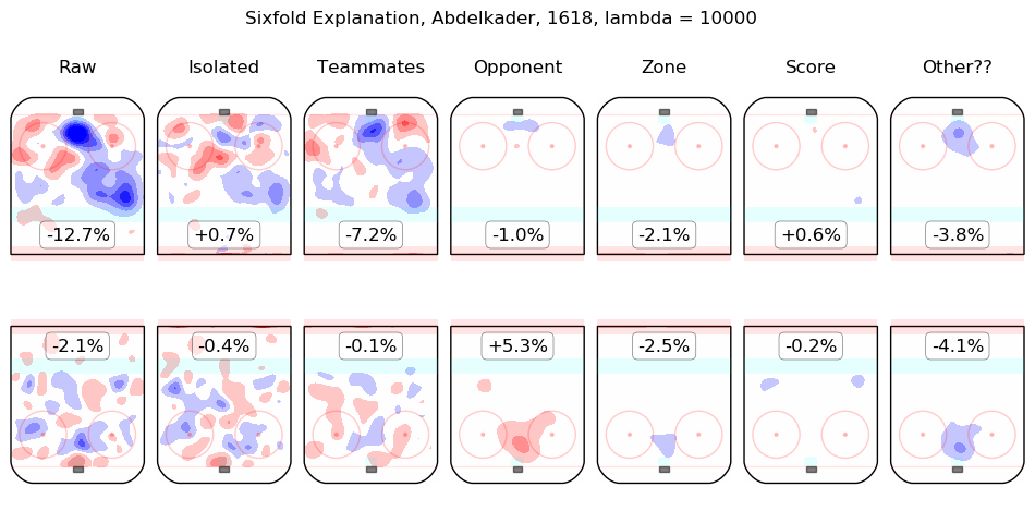
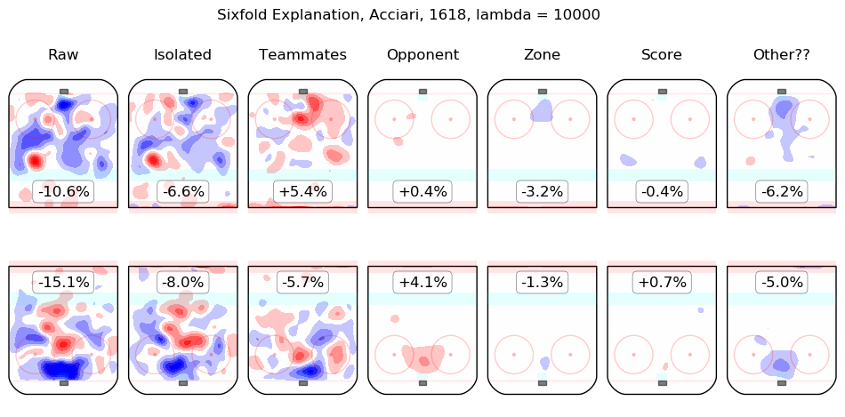
Other skaters may be found alphabetically below: