Estimating Shot Difficulty
This is the updated shooting and goaltending model, which is closely related to the model I introduced last year. Some of the exposition here is copied from that write-up.
Although shots are the basic currency of hockey, it is obvious that not all shots are equally difficult to create, nor equally difficult to score, nor equally dificult to save. The model described here attempts to measure the goal likelihood of various patterns of shots, which is of intrinsic interest, and will also permit us along the way to measure how shooters and goalies can impact goal probabilities.
Vital Theoretical Preliminaries
My animating assumption is that all of the skaters (between six and eleven, in total, usually) are working together both to generate shots for their team and to suppress the generation of shots by the other team. In principle, I consider all of the skaters equally able to affect both processes, in the long run, even if a given skater (for either team) might be only minimally involved with a given shot. All of play in all three zones leading up to and including the decision by a given player to shoot the puck, I understand to be the product of the (combined) ability of all of the skaters, and I call the goal likelihood of shots generated, at the moment the decision to shoot is taken, "expected goal probability", or xG for short. Then, in addition to the xG of the pattern to which a given shot conforms, the shooter themself can, in principle, affect the goal likelihood of the shot, by shooting the puck skilfully, or perhaps (as I might) by woefully butchering whatever chances they and their teammates (and opponents) have conspired to generate. This ability I call "finishing impact" or "shooting talent". Finally, a goaltender can, in principle, affect the goal likelihood of a shot after it is taken, by sneakily interposing their body between the puck and the goal, or, (again as I might do) contriving to fail to do so.
This three-fold division---all of the skaters collectively produce the shot, the shooter shoots, and the goalie endeavours to save---is the animating idea behind the model I describe here. Even at this very basic level these choices have important consequences. For instance a player who is skilled at receiving passes in (relatively) less-dangerous shooting positions and skating untrammelled with the puck to more-dangerous locations will score more often for that reason, and that skill will appear in my accounting in their impact on xG (which will increase, since their team is taking more dangerous shots) and not in their finishing impact (which will presumably decrease, since they are shooting from locations where goals are easier to come by). Similarly, including goaltender effects only on shots already taken prevents us from making any estimate of goaltenders' impact on xG, conceded or generated, from, say, their tendency to handle the puck.
Throughout this article, when I say "shot" I will mean "unblocked shot", that is, goals, saves, and misses (including shots that hit the post or the crossbar).
In contrast to last year's model, which used only 5v5 and 5v4 shots, now I use all shots taken at a net with a goalie, one way or another, as input data.
Odds vs Probability
The machinery here uses the goal odds of a shot throughout, that is, that ratio of the probability of a shot going in the net to the probability of the shot not going in the net. A shot with a goal probability of 50% (that is, of 0.5) has odds of 1, a shot with a goal probability of 20% has odds of 0.20/0.80 = 0.25, and so on. In particular we do not use the word "odds" as if it were a synonym for probability, as if we were craven headline writers.
Method
Once a shot is being taken by a given player from a certain spot against a specific goaltender, I estimate the probability that such a shot will be a goal. This process is modelled with a linear model, and fit with a generalized ridge logistic regression. For a detailed exposition about how such models can be fit, please see Section 5. Briefly: I use a design matrix \(X\) for which every row encodes a shot with the following columns:
- An indicator for the shooter; (in 2019-2020 there were 879 shooters)
- An indicator for the goaltender; (in 2019-2020 there were 86)
- A set of geometric terms and shot types, described below;
- An indicator for "rush shots", that is, shots for which the previous recorded play-by-play event is in a different zone and no more than four seconds prior;
- An indicator for "rebound shots", that is, shots for which the previous recorded play-by-play event is another shot taken by the same team no more than three seconds prior;
- An indicator for teams which are leading and another for teams which are trailing; to be interpreted as representing change in configurations surrounding shots compared to when teams are tied;
- Four indicators for different skater strength situations:
SHfor short-handed shots, that is, ones taken by a team with fewer skaters;PPv3for shots taken by a team with more than three skaters against a team with exactly three skaters;PPfor all other power-play shots, that is, ones taken by a team with more skaters;3v3for play where both teams have exactly three skaters (mostly in overtime)
The Geometric Terms
The various shot types (wrist, slap, backhand, tip, and wraparound) are all qualitatively different in execution and, we observe, arise in different situations. In particular, the pattern of shot locations is quite different for each shot type. Consequently, I choose to model the geometry of each shot type separately. To do so flexibly, consider a hexagonal grid of cells, centred on the split line, covering the offensive zone. To each of the five shot types, I define a "fabric", that is, a subset of these cells which contain at least 95% of all of the shots of that type since 2007-2008. In the process of fitting the model, every shot is assigned to the closest hex in the associated fabric of the shot's type, shown below:
-
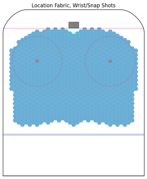 Wrist/Snap shots (734 hexes)
-
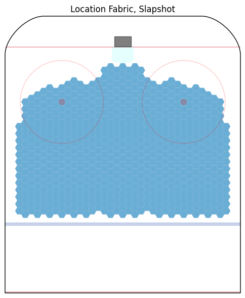 Slap shots (658 hexes)
-
 Backhand shots (433 hexes)
-
 Tips and Deflections (184 hexes)
Each hex in each fabric corresponds to a model covariate, in addition to five indicator covariates for each of the five shot types. The purpose, of course, of making such fabrics is to account for how the goal likelihood of a given shot depends on where the shot is taken. For wraparounds, I found that shot locations clustered very tightly in the two obvious locations (near the goalposts) and that the spatial variation in goal likelihood was extremely small. Thus, I chose to use a simple indicator for wraparounds, without encoding additional geometric detail for those shots.
I especially appreciate Michael Schuckers, who brought the importance of attacking geometric variation separately by shot type to my attention.
For shots recorded as originating below the goal line, I use a single indicator variable; similarly a "neutral zone" indicator for shots originating from behind the blue line. Thus every shot is broken down first by broad location (below goal line, in-zone, or out of zone) and then the in-zone shots are broken down by type, and finally shots of the four main types are tagged with a specific hex in the associated fabric.
Fitting
This section is quite technical and explains the mathematical intricacies of how I fit the above model with NHL data to obtain covariate estimates. If you like you can skip to the results section below. If you read the above section with impatience, you should skip forward; if you read about all those more-than-a-thousand-different hex coordinates and thought "Micah you poor sap this is gonna be overfit to hell and back" you should read this section first.
The observation vector \(Y\) is 1 for goals and 0 for saves or misses. The model itself is the a generalized linear one: $$ Y \sim l\left(X\beta\right) $$ where \(\beta\) is the vector of covariate values and \(X\) is the design matrix described above, and \(l\) is the logistic function $$ x \mapsto l(x) = \frac{1}{1 + \exp(-x)}$$ (extended here to vectors pointwise) after which the regression is named.
Logistic regression coefficient values (the entries of \(\beta\) which we are trying to find) can be difficult to interpret, but negative values always mean "less likely to become a goal" and positive values mean "more likely to become a goal". To compute the goal probability of a shot with a given description (encoded by a particular row \(X_i\) of \(X\); form the sum \(X_i\beta\) of the model covariates to obtain a number, and then apply the logistic function to it to obtain the goal probability.
The logistic function is very convenient for modelling probabilities, since it monotonically takes the midpoint of the number line (that is, zero) to 50% while taking large negative numbers to positive numbers close to zero and very large positive numbers to positive numbers close to one.
The model is fit by maximizing the likelihood of the model, that is, for a given model, form the product of the predicted probabilities for all of the events that did happen (90% chance of a save here times 15% of that goal there, etc.). This product, with one factor for every shot in the data at hand, is called the likelihood, \(L\). Large products are awkward, so instead of maximising \(L\) directly we instead solve the equivalent problem of maximizing the logarithm of the likelihood, denoted by \(\mathcal L\).
Before we compute the covariate values \(\beta\) which minimize the log-likelihood \(\mathcal L\), we bias the results with two so-called ridge penalty terms. These penalty encode our prior knowledge about the terms of the model before we consider the data at hand. The first ridge penalty encodes "static" information (things that we know about hockey generally) and the second one encodes "dynamic" prior information, that is, things learned about the covariates from previous years. By fitting the model with penalties, we obtain estimates which represent a compromise between the data at hand and our pre-existing understanding of what the covariates in the model mean.
Static penalties
The static penalties are encoded as a matrix \(K\) and a term of the form \(\beta^TK\beta\) is subtracted from the overall model likelihood. The entries of \(K\) correspond to pairs of covariates, and we have at our disposal two different types of penalties. We can use diagonal entries \((i,i)\) of \(K\) to penalize large a large covariate value in the \(i\)-th entry, and we can use so-called "fusion" penalties to penalize differences between two specified covariates. In our case we use a diagonal penalty of 100 for each goalie and shooter term, a diagonal penalty of 0.1 for each fabric hex, and a fusion penalty of 5 between each two adjacent hexes. The other terms (the strength indicators, the leading/trailing/rush/rebound indicators, the neutral zone/below goal line/shot type indicators) are unpenalized, so at these terms the model behaves like one fit with ordinary least squares.
It may be helpful to think of attaching elastic bands to each covariate. The diagonal penalties are very strong bands which attach each player value to zero, very weak bands that attach each hex value to zero, and medium-strength bands attaching each hex to its neighbours. Then, after the bands are prepared, the data is permitted to flow in, to push the covariate values while the tension in the bands constrains the resulting fit.
The substantial diagonal penalty for shooters and goalies encodes our prior understanding that all of the shooters and goalies are (by definition) NHL players, whose abilities cannot therefore are understood to be not-too-far from NHL average (that is, zero). The hex penalties work together to allow slow variation in the impact of geometry, encoding our prior belief that shots from nearby locations ought to have similar properties for that reason. In particular, fusing these many hex terms to one another in this way effectively lowers the number of covariates in the model, presumably helping to mitigate over-fitting.
Dynamic Penalties
In addition to the above penalties, I want to suitably accumulate specific knowledge learned from previous years when I form estimates of the impacts of the same factors in the future---in particular we imagine that our estimates for players describe athletic ability, which varies slowly. If you were truly interested only in a single season (or any length of games, thought of as a unity for whatever secret purposes of your own), these dynamic penalties would not be relevant. However, I am interested in fitting this model over each season from 2007-2008 until the present, and so I want to preserve the information gained from each season as I pass to the next. As we shall see, fitting this model produces both a point estimate and an uncertainty estimate for each covariate. The point estimates can be gathered into a vector \(\beta_0\) of expected covariate values, and the uncertainties can be gathered into the diagonal of a matrix \(\Lambda\), and then a penalty $$ (\beta - \beta_0)^T \Lambda (\beta - \beta_0) $$ can be subtracted from the overall likelihood. For players for whom there is no prior (rookies, for instance, but also all players in 2007-2008, since I do not have any data for before that season), I use a prior of 0 (that is, average) with a very mild diagonal penalty of 0.001.
Computational delicacies
In the end, then, the task at hand to fit the model is to discover the covariate values \(\beta\) which maximize the penalized log-likelihood, $$ \mathcal L - \beta^T K \beta - (\beta - \beta_0)^T \Lambda (\beta - \beta_0) $$
Simple formulas for the \(\beta\) which maximixes this penalized likelihood do not seem to exist, but we can still find it by iteratively. (following a very-slightly modified treatment of section 5.2 of these previously mentioned notes): Specfically, beginning with \(\beta_0\) as obtained from prior data (or using the zero vector, where necessary), we will define a way to iteratively obtain a new estimate \(\beta_{n+1}\) from a previous estimate \(\beta_n\). Define \(W_n\) to be the diagonal matrix whose \(i\)-th entry is \( l'(X_i \beta_n) \), where \(X_i\) is the \(i\)-th row of the design matrix \(X\) and \(l'\) is the derivative of the logistic function \(l\) above. Similarly, define \(Y_n\) to be the vector whose \(i\)-th entry is \(l(X_i \beta_n)\). Then define $$ \beta_{n+1} = ( X^TW_nX + \Lambda + K )^{-1} X^T ( W_n X \beta_n + Y - Y_n ) + \Lambda ( X^TW_nX + \Lambda + K )^{-1} \beta_0 $$ Repeating this computation until convergence, we obtain estimates of shooter ability, goaltending ability, with suitable modifications for shot location and type, as well as the score and the skater strength.
Curious readers may wonder if such convergence is guaranteed; it suffices that \(K\) and \(\Lambda\) be positive-definite, which they are.
Results
I have fitted this model to each regular season from 2007-2008 through to 2019-2020;
using the estimates from each summer as the priors to feed into the following year's
regression, as explained above. I explain the results of the 2019-2020 regression in detail
here; historical results can be found via the following links:
2007-2008
2008-2009
2009-2010
2010-2011
2011-2012
2012-2013
2013-2014
2014-2015
2015-2016
2016-2017
2017-2018
2018-2019
Geometry Results
First, the geometric terms, converted to probabilities for display. Each hex is shown with the constant term for that shot type added in already, so that the fabrics can be compared to one another.
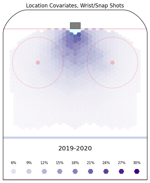
| Wrist/Snap shots. Highest results are in the low slot as expected and drop off sharply outside the dots. |

| Slap shots. Highest in the slot again as expected, but without the sharp drop off side to side and instead falling off roughly with total distance to the net. |
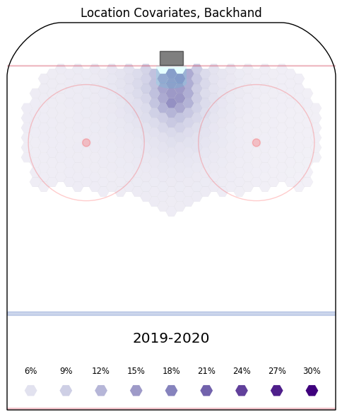
| Backhand shots. High-quality areas are even more tightly concentrated. The bias to the right-hand side of the net is perhaps caused by some combination of an overabundance of left-handed shots with a heavy overabundance of left-catching goaltenders. |
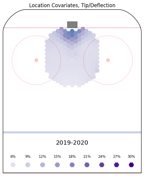
| Tips and Deflections. Again the low slot features best of all, but here the sides of the net are also quite high. |
The base probabilities for:
- shots from below the goal line: 6.2%;
- shots from the neutral zone: 0.4%;
- wraparounds: 4.6%.
Strength, Score, Rush, and Rebound Terms
Since precisely one of the geometric terms above applies to every shot, we can consider them as providing starting odds for us. Then, we can interpret the other covariates in terms of how they modify those odds, so we quote the remaining terms as odds ratios.| Covariate | Impact on Goal Odds |
|---|---|
| SH | +24% |
| 3v3 | +62% |
| PP | +52% |
| PPv3 | +104% |
| Rush | +104% |
| Rebound | +101% |
| Leading | +0.9% |
| Trailing | -7.0% |
Positive values indicate factors that improve the goal odds of a shot, relative to an unadorned even-strength shot. All of the strength terms are considerably positive. Unsurprisingly, we expect that power-play shots, and especially power-play shots facing only three skaters, should have plenty of room in which to fabricate those extra details which we can't measure directly at this time which we nevertheless know make goals more likely; like more time and space to aim and shoot without immediate pressure, more pre-shot movement, and so on. More interestingly, even short-handed shots (rare as they are) have better goal odds than similar even-strength shots.
Rushes and rebounds have associated odds ratios of around double, which accords with our intuition that they make goal odds substantially better. More interestingly, trailing teams shoot worse than tied teams, but leading teams show negligible change for that reason.
Player Results
The model can already be used without specifying shooters or goaltenders, however, this is perhaps a little boring. Below are the values for all the goaltenders who faced at least one shot in the 2019-2020 regular season. I've inverted the scale so that the better performances are at the top. For example, the best goalie this season, Connor Hellebuyck, has a value near -12%, this means that, given an unblocked shot with a goal probability of, say, 9%, corresponding to odds of 0.0989, we estimate that Hellebuck's impact will lower those odds by around twelve per cent, to approximately 0.0883, which corresponds to a probability of 8%. By contrast, Devan Dubnyk, the second-weakest goalie this season, has an estimate of around +14%, his impact on the same shot increases its odds from 0.0989 by fourteen per cent, to 0.113 which corresponds to a probability of 10%.
Similarly for forward and defender results, which I've put on separate pages for performance reasons.
Minimum Shots Faced: