Introduction
I am interested in measuring how the abilities of a given group of athletes change as they age. The exposition here focusses on the National Hockey League, but is applicable to any human activity where we can measure individual ability and where that ability is assumed to change smoothly over time.
This work is a refinement of some of my previous aging work, presented at the Rochester Institute of Technology Sports Analytics Conference in 2019. However, a much more important recent impetus is the preprint of Michael Schuckers, Michael Lopez, and Brian Macdonald, What does not get observed can be used to make age curves stronger: estimating player age curves using regression and imputation. My method here tracks tightly to their method, with one or two deviations.
Method
First, let us specify the set of people whose aging we would like to estimate. I have chosen to consider the set of players who have played at least a thousand minutes of NHL regular-season hockey over the 2007-2023 seasons. This minute threshold serves no technical purpose (the methods here will happily work if one chooses instead, say, all players with at least one shift in the same time period) but instead focusses attention on the kind of players of greater interest to me, namely the ones with non-trivial careers. This cohort comprises 1,548 skaters and 185 goaltenders.
For definiteness, fix a set of ages. I have chosen to use the integer ages of 18 through to 49, inclusive. In point of fact any discrete set of ages can be used. For each of these ages \(a\), we take two model covariates, one \(O_a\) representing the average ability of those players who are Observed in the NHL at age \(a\), and one \(H_a\) representing the average ability of those players who are not observed (that is, are Hidden) in the NHL at age \(a\).
Although a given player in the cohort may not be observed at a given age in the NHL, with vanishingly few exceptions all players who appear in our cohort are observed playing hockey at some reasonably high level (in the AHL, the ECHL, the CHL, the NCAA systems, the KHL, or in any number of european leagues) at nearly every age from their youth up until their retirement. The presence or absence of a given player from the NHL, then, is far from random: a vast network of persons—scouts, stat-keepers, managers, and so on—is employed worldwide to observe our cohort of players and more-or-less deliberately move them from league to league. In short, while the membership of the full cohort itself may be unchanging, the NHL-observed portion of that cohort changes constantly, under selection pressure. Modelling this selection pressure is an important part of properly modelling the aging of the cohort itself.
While the only model covariates are the \(O_a\) and \(H_a\) terms above, they are, strictly speaking, not the desired quantities—we would like the aging of the full cohort. However, we can recover the average ability \(C_a\) of the full cohort at age \(a\) by forming the sum $$C_a = w_aO_a + (1-w_a)H_a$$ where \(w_a\) is the fraction of the cohort observed in the league at age \(a\). This function \(a \mapsto C_a\) is the "aging curve" that we desire.
The observed ability data for each player \(p\) in a given year is encoded in one of three different ways, depending on if the year is an entry year, a departure year, or a middle year. A year is an entry year for a player if they played in that year but not at all in the previous year. A year is a departure year if a player played in that year but not in the following year. A middle year is any year in a player's career that is neither an entry nor a departure year. Every player has at least one entry year and at least one departure year, but players who do not appear for full seasons in the middle of their career will have more than one of both types. Some players do not have any middle years; some years are both entry and departure years.
Middle years are the easiest to encode. For each middle year for a player, we compute the fraction of the year that they were of each age—for instance, a player might have been 28 for 75% of a year and 29 for 25% of the year. These fractions are used as the entries for the corresponding row; so here we would have 0.75 in the column for \(O_{28}\) and 0.25 in the column for \(O_{29}\). The response \(Y\) is the observed ability of the player in that season.
Departure years are handled with more subtlety. To illustrate, suppose a player plays in their age 38 season but does not appear in their age 39 season. We have a measured ability \(Y_{38}\) but we do not have a measured ability \(Y_{39}\). If we did have it, however, we would expect the change \(Y_{38} - Y_{39}\) to be similar to \(O_{38} - O_{39}\), since it is not hard to imagine that the player might have instead continued on to play one more year. Since \(Y_{39}\) does not exist, we replace it with \(H_{39}\), so that we expect \(Y_{38} - H_{39}\) to be similar to \(O_{38} - O_{39}\). Treating this as an algebraic equation to be solved, we can encode \(Y_{38}\) as \(H_{39} + O_{38} - O_{39}\). In this way we synthesize both information about the player's performance in their departure year itself and the fact that it is a departure year. If the observation \(Y\) spans two ages we simply do the above process twice, with suitable weights as above.
Entry years are treated dually, with a result \(Y\) at age \(a\) encoded as \(H_{a-1} + O_a - O_{a-1}\). This encoding pulls \(O_a\) towards the observed results for players of that age but also pulls the estimates of \(O_a\) and \(H_a\) more tightly together for the ages \(a\) in which more players enter or depart the league than for the ages in which they do not.
Imputing Missing Data
For players who are not observed in the NHL in a given year, we consider the obvious question: why not? By definition, every player in the cohort was, or will be, a regular NHL player at some point. There are two obvious reasons: the player no longer wants to play, or, more prevalently, the network of people who decide who does and does not play in the league have made a conscious choice to give the limited minutes that they control to different players. We focus primarily on the latter reason here, though many of the arguments are also somewhat appropriate to the case where players could play but choose not to.
If we assume that the gatekeepers of the league are reasonably attentive and do a capable job of discerning the abilie of the available players in other leagues, then we can trust that there is an effective soft cap on the ability of the players that we do not observe. On the one hand, we know that the player is not very far away in ability from the others, since they are NHL regulars at some point in their career. However, they cannot be among the very best players at their age, since they are being observed by a network of people who are endeavouring to put the very best players into the NHL, and the various logistical difficulties (salary cap exigencies, waiver statuses, plane flights, visa rules, machinations of international diplomacy) of doing so, while no doubt a source of trouble to those immediately concerned, are by no means insurmountable in the aggregate.
We resolve this tension in the following way: for a player who is not observed in a given season, we impute a value for what their ability by drawing a random value from a normal distribution whose mean is the mean of the abilities for players at that age who are observed, but then reject the sampled value if it is above the 75th percentile of that distribution—if the player's ability were so high, we assume that they would somehow be put into the league. This method, as well as the rejection threshold, are both taken from the preprint of Schuckers, Lopez, and Macdonald above. The standard deviation of this notional distribution from which we sample is computed from the standard deviation of the observed abilities and the fraction of the cohort which is observed at the age at hand, again following their method.
This imputation step is where we explicitly model the (aggregate) behaviour not of the players, but of the network of gatekeepers who decide which players comprise the league. If we imagined that these persons were extremely good at their jobs, we would move the 75th percentile threshold lower; if we imagined that their decisions were entirely random, we might move the threshold to something much higher—if it were raised arbtirary high that would corespond to there being no distinction in quality between the players in and out of the top league at any given age.
In a future version of this work, I mean to replace this imputation method with a more sophisticated one, possibly considering in more detail the reasons why a given player might or might not be chosen to play in the NHL, such as the specific age they happen to be, their nationality, the pathway their previous career has taken, their positions, perhaps even their family kinship to previous NHL players or their ethnicity. This sort of sophistication is evidently a more delicate matter than the somewhat drier work of modelling on-ice behaviour only.
Fitting
This model is fitted using ordinary least squares fitting, but with three kinds of ridge penalties, similar to my shot rate model. Typically, penalties are restricted to diagonal ones, that is, encoding a prior belief that covariate values are not far from zero. Here, we do not use any such penalties, and instead use so-called "fusion" penalties. In their most general forms, such penalties encode a prior belief that a given linear combination of model terms should be close to zero. The simplest fusion penalties are the ones that pull two terms together (by asking that the square of the difference between the two terms should be close to zero). We use two such schemes of penalties, fusing \(O_a\) to \(O_{a+1}\) and \(H_a\) to \(H_{a+1}\) with strengths proportional to the fraction of players of the cohort who are shared between the two ages.
The derived terms \(C_a = w_aO_a + (1-w_a)H_a\), though, are the terms of true interest, and the only ones supported by the full cohort of players. Specifically, we expect that \(C_a\) will vary smoothly as a function of \(a\), since we know that the physical changes that occur in the adult human body as it ages are gradual. To do this, we ask that \(C_a\) be similar to \(C_{a+1}\) by asking that the square of \( w_aO_a + (1-w_a)H_a - w_{a+1}O_{a+1} - (1-w_{a+1})H_{a+1} \) should be close to zero.
All of these penalties are multiplied by a constant factor of fifty thousand, this is empirically chosen to give a suitably smooth result.
I have access to data from 2007-2008 through to 2022-2023; I use all seasons in order to determine who has or has not played a thousand minutes, and for discerning which seasons are entry/departure/middle seasons. However, I do not use the data from the 2007-2008 season (since it would be labourious to determine which players are entering the season that year) nor from 2022-2023 (since it is in progress).
Following Schuckers, Lopez, and Macdonald, I use a multi-step process to produce the final fit:
- Impute the missing data using the mean observed values.
- Fit the model as described.
- Discard the old imputed data, re-impute it using the full cohort estimated mean.
- Fit the model as described, again.
Results
Even-Strength Shot Rate Results
Until now we have talked only of "ability" without specifying precisely what ability we are talking about. This is deliberate, since the framework described above will be appropriate for any ability for which we have a measurement that we trust is suitably isolated to the individual. In particular, I can use as the ability measure my even-strength shot rate model, which estimates, among other things, the impact of each player on their team's shot generation and suppression.
For shot generation, the results are as follows:

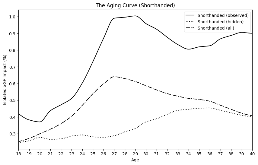
Here the solid line is the model coefficients \(O_a\), and the dotted line is the model coefficients \(H_a\). The dot-dashed line between them is the "aging curve" of \(C_a = w_aO_a + (1-w_a)H_a \). The zero line here is the observed NHL mediant play; the aging curve of the full cohort is entirely below that, as we expect. If we were to confine ourselves purely to observed data, we would erronneously conclude that the peak age for this skill is nineteen or twenty; in fact players of that age who play in the league do so almost entirely because their coaches and managers are already quite sure that they will be very good, and have usually quite recently drafted them for just such a purpose. The observed upwards slope at high ages is also due to selection bias, as the better players remain and the weaker ones retire or are replaced.
For shot suppression, the results are as follows:
Here I've negated the values, so that the observed curve peaks near 1%, that is, 1% of league average shots suppressed. Here we see a broadly similar pattern to offence, with players improving relatively quickly until the age of 25, and then a more shallow decline. In fact, all abilities in this article have been negated where appropriate so that the more desirable impacts are "up" on every graph.
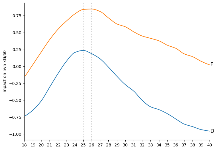
Putting both curves on the same axis helps compare the two facets:
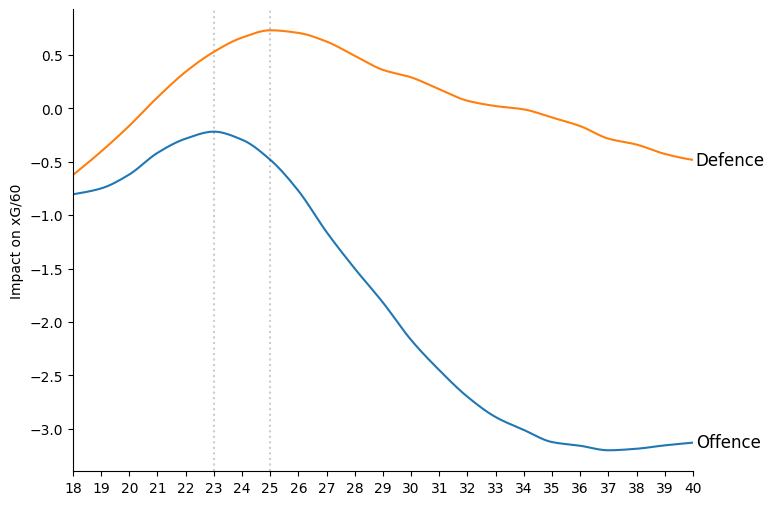
Not only does defensive suppression peak later, it is, comparing like ages, always higher than offensive creation and falls off much more slowly as players age.
Special Teams Shot Rate Results
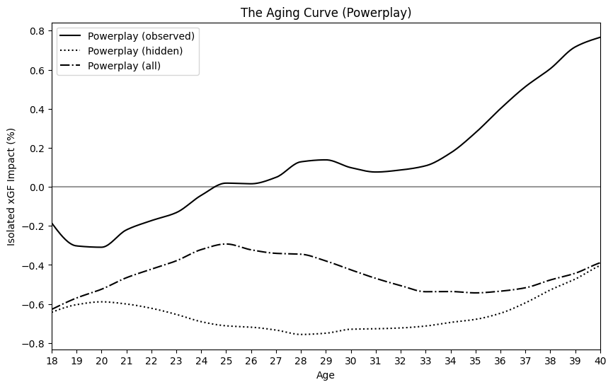
The same process can be repeated with different abilities; such as individual isolated impact on power-play shot generation and short-handed shot suppression, which I measure using my special teams shot rate model.For powerplay shot generation, the results are as follows:
For shorthanded shot suppression, the results are as follows:
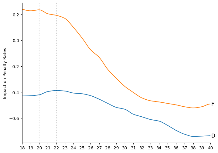
Putting both curves on the same axis helps compare the two facets:
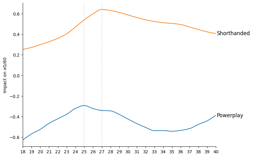
Here, just as in the even-strength case, the defensive aspect of the game is stronger at each age, and also peaks a couple years later, but the peak ages are later. The uptick in the power-play ability may be a modelling artifact, or it may be players deliberately honing their powerplay skills late in their careers in order to remain in the league.
Since special teams minutes are scarce and high-leverage, they are subject to a further level of selection. This makes the plain 'observed' results an even less reliable guide to how players age. Older players with established power-play ability routinely continue to play such minutes even as they lose even-strength resources (minutes and higher-quality teammates). If we did not control for selection effects we would be badly misled.
Penalty Drawing and Taking
I also have a penalty model, which estimates, among other things, the tendancy of a player to cause their team to take or to draw penalties.For impact on drawn penalties, the results are as follows:
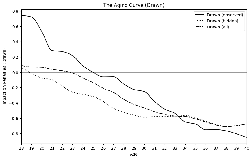
Notice here something unusual: the curves for the hidden cohort and full cohort rise above the observed, despite the truncation in the imputation we use. This is caused by the smoothing penalties that we enforce.
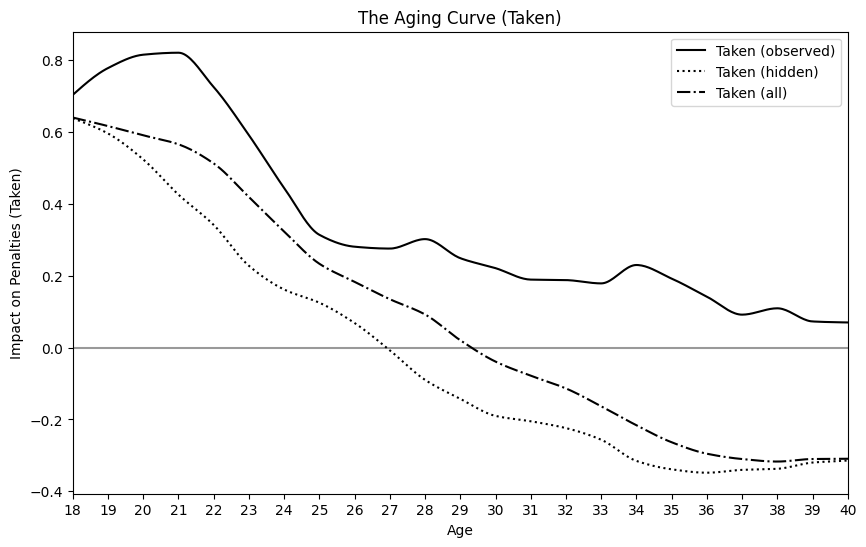
For impact on taken penalties, the results are as follows:
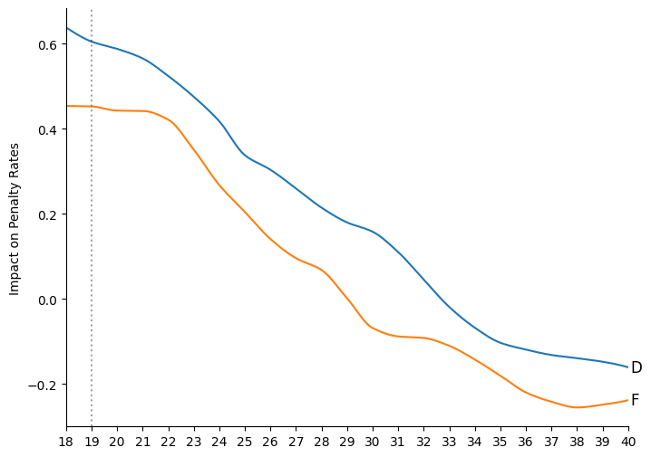
Putting both curves on the same axis helps compare the two facets:
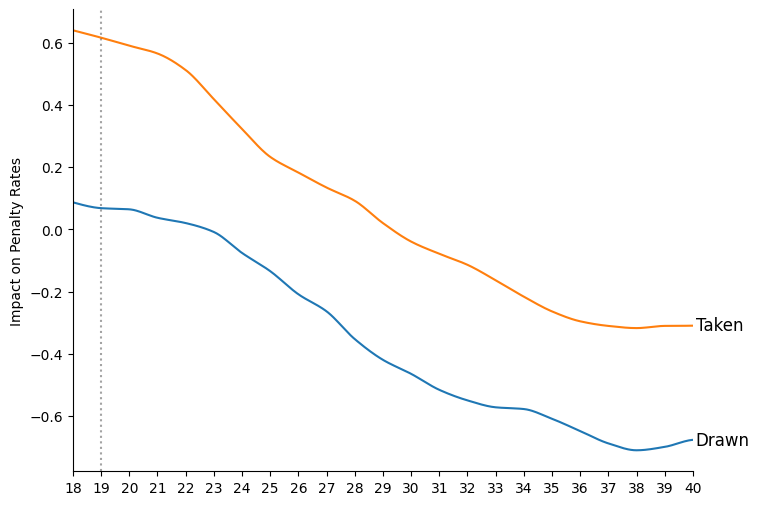
Here the "typical" shape of the aging curve is absent; both the ability cause one's team to draw penalties and the ability to prevent one's team from taking penalties are highest for the youngest ages and decline more or less uniformly as players age. Interestingly, the difference between the two curves appears to be constant over most ages. I have a suspicion that this is because the most important factor, both to drawing penalties and to making sure that one does not commit them, is footspeed.
Notice again that the defensive ability (that is, impact on penalties taken, the one where it is desired that the thing not happen) is above the offensive ability once again.
Goal Impact Stats
Finally, there is a trio of stats the naturally group together into what I call "goal threat", that is, the ability of individual players to make shots more or less likely to become goals. These are finishing (the ability of the shooter to get the puck past the goaltender), setting (the ability of the person passing the puck to the shooter to do so skillfully) and goaltending. I measure these abilities with my xG model.For finishing, the results are as follows:

For setting, the results are as follows:

For goaltending, the results are as follows:

Putting both curves on the same axis helps compare the three facets:
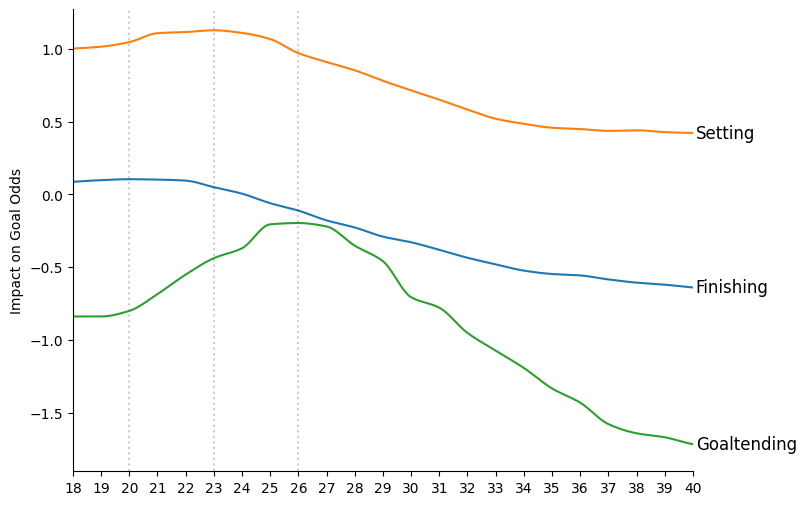
The goaltending curve has the most "typical" shape, with a peak age at 26, older than the peak of most skater abilities. More interestingly, the early part of the finishing and settings curves are both very flat, suggesting that by the time skaters enter the league their goal threat abilities are more or less already fully developed.
Appendix: Positional Breakdown
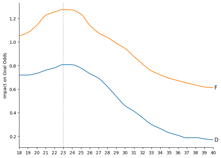
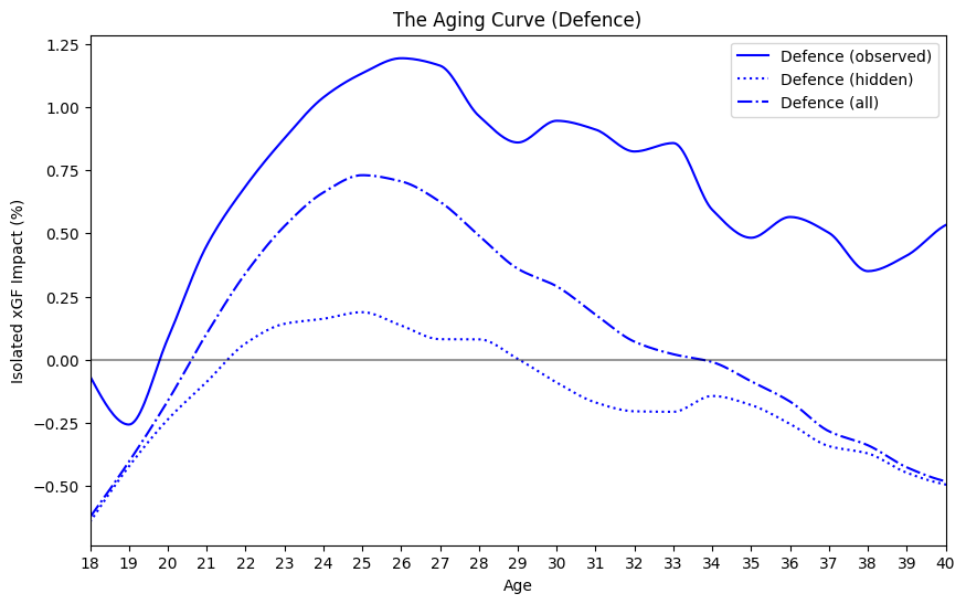
For each of the skater abilities, the above process can be repeated, but using only defenders or only forwards. The results are as follows:
Offence

Defence
Powerplay

Shorthanded

Drawn
Taken
Finishing

Setting